Energy efficient cooperative mobile sensor network
Bạn đang xem bản rút gọn của tài liệu. Xem và tải ngay bản đầy đủ của tài liệu tại đây (3.73 MB, 235 trang )
ENERGY EFFICIENT COOPERATIVE
MOBILE SENSOR NETWORK
MAR CHOONG HOCK
(B.ENG. (HONS, FIRST CLASS), NUS,
M.ENG., NUS)
A THESIS SUBMITTED
FOR THE DEGREE OF DOCTOR OF PHILOSOPHY
NUS GRADUATE SCHOOL FOR INTEGRATIVE
SCIENCES AND ENGINEERING
NATIONAL UNIVERSITY OF SINGAPORE
2008
i
Acknowledgements
First, I thank Agency for Science, Technology and Research (A*STAR) for
granting me the A*STAR Graduate Scholarship (AGS) to pursue my PhD research.
Second, I thank my supervisor, Dr Winston Seah, for the supervision and
guidance. Also I thank both members of the Thesis Advisory Committee for taking
time off their schedules to give me insightful feedback. In particular, I thank Prof Lye
Kin Mun for his gems of wisdom and kind advice and A. Prof Ang Marcelo H. Jr. for
his gentle encouragement and support.
Third, I thank my loved ones: my wife, Chiew Pei and siblings (Ling Ling and
Chong Kiat) for the many joyful moments and emotional supports in my long tedious
journey of PhD research.
Fourth, I thank my endearing lab mates: Liu Zheng, Hwee Xian, Inn Inn,
Ricky, Junxia, etc for giving me many wonderful moments in the lab and enrich my
otherwise prosaic PhD life.
Finally, I thank my former supervisor, Prof Kam Pooi Yuen and those people
who have at one time or another gracefully extended both their helping hands and
sympathetic ears to me. Although those people remain anonymous in this page, I
remember their kindness.
ii
Table of Content
SUMMARY IV
LIST OF TABLES VI
LIST OF FIGURES VII
LIST OF ABBREVIATIONS IX
LIST OF NOTATIONS X
LIST OF PUBLICATIONS XIII
CHAPTER 1: INTRODUCTION 1
1.1 BACKGROUND AND CONTEXT 1
1.2 RESEARCH PROBLEM 6
1.3 SIGNIFICANCE AND CONTRIBUTIONS OF OUR RESEARCH 7
1.4 ADVANTAGES OF MOBILE SENSOR NETWORK 9
1.5 METHODOLOGY 14
1.6 RESEARCH SCOPE, AIMS AND OBJECTIVES 14
1.7 ORGANIZATION OF THE THESIS 16
CHAPTER 2: LITERATURE SURVEY 18
2.1 MOBILE AD-HOC NETWORKS 18
2.2 WIRELESS SENSOR NETWORKS 24
2.3 MOBILE SENSOR NETWORKS 32
2.4 CONCLUSION 38
CHAPTER 3: PRELIMINARY INVESTIGATION AND ANALYSIS 40
3.1 CONNECTIVITY ANALYSIS OF A MANET OF COOPERATIVE AUTONOMOUS MOBILE AGENTS40
3.1.1 The Method 41
3.1.2 Numerical and Simulation Results 42
3.1.3 Conclusion 44
3.2 CSMA/CA THROUGHPUT ANALYSIS OF A MANET OF COOPERATIVE AUTONOMOUS MOBILE
AGENTS UNDER THE
RAYLEIGH FADING CHANNEL 45
3.2.1 Method 47
3.2.2 Numerical and Simulation Results 54
3.2.3 Conclusion 60
3.3 DS/CDMA THROUGHPUT OF MULTI-HOP SENSOR NETWORK IN A RAYLEIGH FADING
UNDERWATER ACOUSTIC CHANNEL 61
3.3.1 Methods 62
3.3.2 Numerical and Simulation Results 65
3.3.3 Conclusion 67
3.4 CONCLUSION 68
CHAPTER 4: THE COOPERATIVE CONTROL ALGORITHM 70
4.1 GENERAL OVERVIEW 70
4.1.1 Organization of the Mobile Sensor Group 70
4.1.2 Motion Control 74
4.1.3 Information Processing 75
4.2 THE ALGORITHM 77
4.2.1 Cooperative Optimal Placements 79
4.2.2 Independent Optimal Harvesting 104
4.2.3 Tracking Mechanism 113
4.2.4 Our Research Contributions 123
4.3 THEORETICAL PERSPECTIVE ON OUR DESIGN 125
4.4 CONCLUSION 126
iii
CHAPTER 5: PERFORMANCE STUDIES 128
5.1 GENERAL OVERVIEW 128
5.1.1 Simulation Setup 128
5.1.2 Assumptions 135
5.1.3 Metrics 137
5.1.4 Simulation Parameters 139
5.2 COMPARATIVE STUDY 140
5.2.1 Relative Performance with Mobile Sensor Networks using different harvesting
algorithms 140
5.2.2 Relative Performance with Static Sensor Networks 150
5.3 STABILITY STUDY 153
5.3.1 Optimization Stability 153
5.3.2 Tracking Stability 158
5.4 THE EFFECT OF NON-IDEAL COMMUNICATIONS AND SENSOR FAILURES 159
5.4.1 Effect of non-ideal communications 159
5.4.2 Effect of sensor failures 163
5.5 CONCLUSION 164
CHAPTER 6: CONCLUSION 166
6.1 FUTURE WORK 170
APPENDIX A: CSMA/CA THOUGHPUT ANALYSIS OF A MANET OF COOPERATIVE
AUTONOMOUS MOBILE AGENTS UNDER THE RAYLEIGH FADING CHANNEL 173
APPENDIX B: DERIVATION OF THE MOTION CONTROL EQUATIONS FOR ONE-
DIMENSIONAL TOPOLOGY 183
APPENDIX C: DERIVATION OF THE MOTION CONTROL EQUATIONS FOR TWO-
DIMENSIONAL TOPOLOGY 191
APPENDIX D: STABILITY ANALYSIS OF OPTIMIZATION 204
APPENDIX E: STABILITY ANALYSIS OF TRACKING MECHANISM 209
REFERENCE 212
iv
Summary
We research into the challenge of improving the quality of the reconstructed
distribution from spatiotemporal monitoring data collected by mobile sensor network.
Our approach is to attack the problem from the source, by mobilizing the sensors to
harvest data of high information content so that the reconstructed distribution has
minimum distortion. We consider four realistic constraints in our design: limitations
of wireless communications, limited supply of energy and sensor resources and
difficult terrains. Our strategy is to treat each mobile sensor as an intelligent
cooperative autonomous agent, capable of processing cooperative shared information
independently in order to carry out its harvesting task in an optimal manner. In the
greater scheme, the sensors are to be divided into small self-contained cooperative
groups for two reasons. First, it improves scalability and facilitates deployment in
difficult terrains partitioned by obstacles. Second, it is more robust to communication
problems since communications used to facilitate the harvesting tasks are intra-group
in nature.
We investigate into the limitations in wireless communications through
literature surveys and theoretical analyses. In our analysis, we examine better
approaches to organize sensors and design our algorithm so as to alleviate the three
main communication problems at the topological, Medium Access Control (MAC)
and routing layers. We conclude that the sensors should move orderly where same
neighbors are maintained in the neighborhood to prevent routing breakages. Inter-
group and multi-hop communications should be minimized. They are taken into
consideration in the design of the dissemination protocol of our algorithm.
v
In our comparative study, we compare the performances of the following
using relative global error and total energy consumption: three versions of our
cooperative algorithm (cooperative, cooperative-delta and cooperative-orbital
harvesting), mobile sensors deployed in Equally Distributed Grid (EDG), three types
of independent methods (Broyden-Fletcher-Goldfarb-Shanno, Random Waypoint and
our independent delta-harvesting) and static sensors. Our simulation results show that
cooperative-orbital algorithm outperforms others. It reduces an average of 738% (with
a range of 625% to 885%) more error than mobile sensors deployed in EDG and 35-
314% more error than independent methods by consuming 74-81% lesser energy. Our
method also has a resource utilization efficiency of 250 times that of static sensors.
In our stability study, we show that the following two methods improve the
robustness of optimization: incorporation of an independence phase in our algorithm
and division of a group into smaller groups. Therefore, the division of a group into
smaller groups has three benefits: easy deployment in difficult terrains, robust
communications and stable cooperation. Moreover, we show that our tracking
mechanism is stable and the performance is robust against non-ideal communications
and sensor failures.
Finally, we have five research contributions. In the optimization mechanism of
the algorithm, we adapt the pseudo-Newton algorithm and make four improvements
to it as follows: adaptive cooperative search goals in optimization, local RBF
interpolation in estimations, dissemination to mitigate the initial value problem and
the concept of orientation stabilization to provide adaptive stabilized search direction.
Our fifth contribution is the adaptation of the dynamic clustering technique to track
continuous distribution robustly.
vi
List of Tables
Table Title Page
3.1 Abbreviations in timing diagram 48
3.2 Values for the common parameters used in the throughput
simulation of a MANET using CSMA/CA and AODV protocols
55
5.1 Values of the parameters for the performance studies 138
5.2 Relative performance of cooperative-orbital algorithm 144
vii
List of Figures
Figure Title Page
1.1 Three possible applications 4
1.2 Vast oceanic mobile sensor network 5
1.3 Forest fire scenario 7
1.4 The invariance property of Delaunay graph for coordinated
movements
13
1.5 Achieving global connectivity by maintaining local connectivity 13
2.1 Interference in a multi-hop network 19
2.2 Three different approaches in active routing 22
2.3 Minimum covering set 27
2.4 Data clustering and aggregation 28
2.5 Maximum area covered by a mobile node in its search 29
3.1 Study on the effects of varying the transmission range and node
count on the connectivity probability
43
3.2 Timing diagram for a successful transmission followed by a failed
transmission
48
3.3 Expanding ring search for the first two tries 50
3.4 Results for the throughput simulation of a MANET using
CSMA/CA and AODV protocols
56
3.5 Sensor network model 62
3.6 State diagram for the synchronous half-duplex control protocol 64
3.7 Results for the throughput simulation of an UWA multi-hop Sensor
Network using DS/CDMA and AODV protocols
66
4.1 Different ways of organizing our mobile sensor group 71
4.2 Cooperative optimal control block 74
4.3 The high-level framework of our algorithm 78
4.4 The main cooperative control algorithm 79
4.5 Quality enhanced reconstructed distribution map using pptimally
spaced sensors
80
4.6 Local distortion metrics 80
4.7 Distortion Error 84
4.8 Optimum condition of minimum distortion error 86
4.9 Neighborhood couplings 87
4.10a Dissemination mechanism (S4) 99
4.10b Extraction mechanism (S1) 99
4.11a An example of a trajectory plot of the movements of the 25 mobile
sensors without orientation stabilization
101
4.11b An example of trajectory plot of the movements of the 49 mobile
sensors with orientation stabilization
101
4.12a An example of trajectory plot of the movements of 4 groups of 25
mobile sensors without information dissemination for the first 7
iterations
102
4.12b An example of trajectory plot of the movements of 4 groups of 25 102
viii
mobile sensors with information dissemination for the first 7
iterations
4.13 Pseudo-code for the coordination protocol 106
4.14a The trajectory for the delta-harvesting heuristic 107
4.14b Pseudo-code for the main function of the delta-harvesting heuristic 108
4.14c Pseudo-code for the recursive function of the delta-harvesting
heuristic
109
4.14d Pseudo-code for the adaptive step size function of the delta-
harvesting heuristic
110
4.15a The trajectory for the orbital-harvesting heuristic 111
4.15b Pseudo-code for the orbital-harvesting heuristic 112
4.16a Format of communication packet 113
4.16b Dynamic clustering algorithm 114
4.17 Tracking algorithm 116
4.18 Stability condition during tracking 117
4.19 Crossover condition of hotspots and handover effect of tracking
algorithm
118
4.20 Blind spot problem 120
4.21 Cluster-head peak search algorithm 121
5.1 Scenarios with hills and valleys of irregular shapes 128
5.2 Scenarios with 4 hotspots 129
5.3 Scenarios with 8 hotspots 130
5.4 Five-point stencil maneuver 132
5.5 Trajectory plot of 9 sensors using the independent delta-heuristic 133
5.6a Relative global errors for the different algorithms for the 9
scenarios
139
5.6b Total energy consumption per sensor for the different algorithms
for the 9 scenarios
140
5.7 Reconstructed distributions of scenarios with hills and valleys of
irregular shapes using data obtained from cooperative-orbital
algorithm
146
5.8 Reconstructed distributions of scenarios with 4 hotspots using data
obtained from cooperative-orbital algorithm
147
5.9 Reconstructed distributions of scenarios with 8 hotspots using data
obtained from cooperative-orbital algorithm
148
5.10 Relative global error of static sensor network 151
5.11a Error spread for different methods 153
5.11b Energy consumption spread for different methods 155
5.12 Average separations between the centers of the tracking clusters
and the hotspots
158
5.13 Relative global errors for the terrestrial and underwater DS/CDMA
communications scenarios
160
5.14 Beneficial diversity effect when there are more than three network
neighbors
161
5.15 Effect of sensor failures on the error reduction performance 162
ix
List of Abbreviations
Abbreviation Description
1D One-dimensional
2D Two-dimensional
3D Three-dimensional
AODV Ad Hoc On-Demand Distance Vector
AWGN Additive White Gaussian Noise
BFGS Broyden-Fletcher-Goldfarb-Shanno
CSMA/CA Carrier Sense Multiple Access with Collision Avoidance
DS/CDMA Direct Sequence Code Division Multiple Access
EDG Equally Distributed Grid
ERC Equal Ratio Combining
FIFO First-In-First-Out
GPS Global Positioning System
LDM Local Delaunay Map
LHS Left hand side
MAC Medium Access Control
MANET Mobile Ad-Hoc Network
MAI Multi-Access Interference
MRC Maximal Ratio Combining
PMM Probabilistic Mobility Model
RHS Right hand side
RWM Random Waypoint Mobility
RBF Radial Basis Function
RWMM Random Walk Mobility Model
SLAM Simultaneous Localization and Mapping
TDMA Time Division Multiple Access
UWA Underwater Acoustic
WLAN Wireless Local Area Network
WSN Wireless Sensor Network
i.i.d. Independently and identically distributed
r.m.s. Root mean square
s.t. Such that
w.r.t. With respect to
x
List of Notations
Notation Description
c
ab
, c
link
Connectivity Probability between two nodes: a and b
c
a
Average Connectivity Probability of a node a, with any nodes
N, N
s
Number of nodes in the terrain
R
ab
Euclidean distance between two nodes: a and b
S
The length of the square region used in the connectivity
analysis expressed in integer number of steps
(x
a
, y
a
) Cartesian coordinate of node a
aa
yx
π
π
Stationary Position probability of node a
S(M,
λ
)
Normalized MAC throughput used in the throughput analysis
M
Number of nodes in a one-hop network neighborhood
λ
Offered Traffic Load
π
i
(M,
λ
)
Stationary probability distribution of the backlogged node
P
s
(i,
λ
)
Probability of successful packet transmissions given i
backlogged nodes
i
I
Average idle period in the channel given given i backlogged
nodes
T
p
Packet transmission duration
Φ
Average number of neighbors
G
eff
Effective offered load
P
MAI
The probability that a packet is successfully modulated in the
presence of Multi-Access Interference in DS/CDMA
P
RS
The probability that a packet is successfully received in the
Receive state of the MAC protocol
)(k
i
p
The position of sensor i in the k
th
time step. Sometimes, it is
expressed in Cartesian coordinate form
(
)
)()(
,
k
i
k
i
yx .
)(k
i
θ
The measurement made by sensor
i in position
)(k
i
p in the k
th
time step.
)(k
i
s
The state vector of sensor
i in the k
th
time step. It is defined as
the concatenation of
)(k
i
p and
)(k
i
θ
. ],[
)()()( k
i
k
i
k
i
ps
θ
=
∴
.
)(k
sn
C
The set that represents the states of the sensors belonging to
the same cooperative group in the
k
th
time step.
(
)
)(
)(
k
sn
k
i
CpΔ
This is the position control function in the k
th
time step. It takes
)(k
sn
C
as the input and computes the amount of adjustment to
be added to the current position,
)(k
i
p
in order to obtain the
next position.
)(
,
k
sni
V
The set that represents the states of the Voronoi neighbors of
sensor i in the k
th
time step, exclusive of sensor i.
)(k
i
LA
The local area of sensor i in the k
th
time step.
xi
)(k
p
LA
i
i
∂
∂
The first derivative of local area of sensor i in the k
th
time step.
We also denote it as
(
)
kpy
i
, for clarity of presentation. That
is,
()
)(, k
p
LA
kpy
i
i
i
∂
∂
= .
)(k
p
i
i
∂
∂
θ
The first derivative of sensed value
θ
i
of sensor i in the k
th
time
step.
)(
2
2
k
p
i
i
∂
∂
θ
The second derivative of sensed value
θ
i
of sensor i in the k
th
time step.
u
goal
Goal function
D
e
Distortion error metric
K
u
Control gain
V
Volume of the tetrahedron
A, B and C Areas of the triangle projection of the base of the tetrahedron
constructed from the four points representing the state
information of the four sensors: (x
i
, y
i
,
θ
i
), (x
1
, y
1
,
θ
1
), (x
2
, y
2
,
θ
2
) and (x
3
, y
3
,
θ
3
)
g(k) Gradient of V
H(k) Hessian of V
∇
θ
i
(k)
Gradient of temperature of node i computed at the k
th
time step
∇
2
θ
i
(k)
Gradient of temperature of node i computed at the k
th
time step
I
n
n × n Identity Matrix
•
2-Norm (Magnitude) of the Vector
•
The matrix determinant. For scalar, it evaluates to the absolute
value.
)(
h
pp −
ϕ
Radial Basis Function. p
h
is a known position. p is the position
of interest. We want interpolate (estimate) the temperature at
position p
Φ
Interpolation matrix, used in RBF interpolation.
θ
Interpolation temperature vector containing all the known
temperature
w
Interpolation weight vector
σ
RBF constant, usually set to a large value for smooth
interpolation
D
ij
Directional gradient pointing from point i to j
u
ij
Unit directional vector pointing from point i to j
D
st
Steering direction
u
st
Unit steering direction
ε
p
Mean location error
ε
θ
Mean temperature error
)(k
i
pΔ
Computed change in position
)(
,
k
sti
pΔ
Computed change in position stabilized by u
st
)(
ω
Ψ An approximate distribution interpolation using the cubic
spline function available in MATLAB.
ω
is the spacing of the
known sampling points
ξ
(k)
Relative global error computed at the k
th
time step
xii
E(k)
Energy consumption per sensor computed at the k
th
time step
h
The computation interval used to compute the relative global
error
σ
max
Maximum separation between the hotspot and the tracking
cluster
T
0
Total delay in sensor response
T
comm
Communication delay
T
θ
Measurement delay of the thermometer
S
data
Data throughput
N
hops
Maximum number of hops by the data packet to reach
destination
V
s
Maximum velocity of the sensor
V
h
Maximum velocity of the hotspot
m
s
Mass of the sensor
u
f
Coefficient of friction
φ
Angle of deviation used in the orbital harvesting heuristic
xiii
List of Publications
P1. C. H. Mar and W. K. G. Seah, “An analysis of connectivity in a MANET of
autonomous cooperative mobile agents under the Rayleigh fading channel,”
Proceedings of the IEEE 61
st
Semiannual Vehicular Technology Conference,
Spring 2005, Stockholm, Sweden, May 30- Jun 1, 2005, vol. 4, pp. 2606-10.
P2.
C.H. Mar and W.K.G. Seah, “DS/CDMA throughput of multi-hop sensor
network in a Rayleigh fading underwater acoustic channel,” Proceedings of
the 20th International Conference on Advanced Information Networking and
Applications, Vienna, Austria, Apr 18-20, 2006, vol. 2.
P3.
C.H. Mar and W.K.G. Seah, “DS/CDMA throughput of multi-hop sensor
network in a Rayleigh fading underwater acoustic channel,” Concurrency:
Practice and Experience, vol. 12, no. 6, pp. 1129-40.
P4.
C.H. Mar, W.K.G. Seah, K.M. Lye and Ang H Jr. Marcelo, “An Energy
Efficient Cooperative Optimal Harvesting Algorithm for Mobile Sensor
Networks,” Proceedings of IEEE 19
th
International Symposium on Personal,
Indoor and Mobile Radio Communications, Cannes, France, Sep 15-18, 2008.
P5.
C.H. Mar, W.K.G. Seah, K.M. Lye and Ang H Jr. Marcelo, “Robust
Cooperative Data Harvesting Algorithm for Mobile Sensor Networks under
Lossy Communications,” Pending Submission to IEEE Transactions on
Systems, Man, and Cybernetics.
xiv
This page is intentionally
left blank.
1
Chapter 1: Introduction
This thesis is a report on the development of our cooperative control algorithm
for the mobile sensors to optimize the harvesting of spatial environmental information
with four realistic constraints: limitations of wireless communications, limited supply
of energy and sensor resources and to a lesser extent, difficult terrains. The algorithm
is inspired partially by nature [1][2] and draws upon the principles from an eclectic
mix of cooperation [1]-[4], optimal control [5][6] and statistical decision theories. The
following is presented in this chapter. In section 1.1, we describe the background and
context of the research. In section 1.2, we specify our research problem. In section
1.3, we enumerate on the significance and contributions of our research. In section
1.4, we justify our use of mobile sensors instead of static sensors in terms of
advantages gained. In section 1.5, we present an overview of the methodology used to
solve our research problem. In section 1.6, we outline our research scope and aim and
breakdown each aim into several objectives to be attained in this research. Finally, in
section 1.7, we present the overall organization of this thesis.
1.1 Background and Context
The rapid research and technological advances in wireless communications,
sensors and actuators have created exciting and innovative ways of using them that
we have never seen before. We envisage a near future where the seamless integration
of the abovementioned technologies and devices can make us understand our world
better and a safer, efficient and greener place for us to live in. However, many
challenges lay ahead, both within each field and in the integration of the fields of
2
research. In the areas of wireless communications, we have challenges ranging from
connectivity and reliable communications in the networks due to poor fading channels
to security of the networks. In the areas of wireless sensors, challenges typically
originated from the paucity of two basic sensors resources: communication bandwidth
and energy. Recently, we also witness new fields of research which involved creating
smart autonomous actuating devices and robots that can adapt their behaviors
according to time-varying sensory inputs. Within these wide overarching research
concerns lay our research interest.
In recent years, there is an increasing number of research problems related to
the deployment of Wireless Sensor Networks (WSN) [7]-[14][P2][P3] in diverse
environments to measure environmental data. These data represent physical quantities
that emanate from sources and are diffused in space. For our research, we focus on the
use of Mobile Sensor Networks [15]-[20] to harvest such data in an optimal manner
so that quality information can be extracted from them. Mobile sensors are sensors
that are mounted on vehicular platforms, which could either be land, sea or air based.
Thus, they are capable of changing their positions adaptively based on either changes
in the topology (for example, due to failed sensors) or internal states of the sensors
(for example, low power) or explicit commands from a command centre. Hence, they
are more versatile than static sensors. For example, they can be programmed to
automatically return to a collection point when they accomplish their mission or when
their batteries need to be recharged. Static networks are onerous to gather for disposal
or redeployment especially when the sensors are deployed in large quantity in dense
vegetations, seabed or hazardous environments. In the long run, battery leaks from
uncollected sensors can cause pollutions. However, mobile networks are usually
deployed at lower node densities with equal spacing [15]-[18]. As a result, the
3
reconstructed distribution maps are highly distorted and significant amount of post-
processing is required to enhance the quality of collected data.
Our networks are to be deployed in environments that are either hazardous or
impossible for human intervention. In the future, we believe that many novel
applications in the areas of scientific monitoring and disaster management can
germinate from such a research. For example, scientists who place high premiums on
high quality experimental data to confirm their hypothesis and theoretical models in
their quest to unravel the mystery of nature will find such harvested data valuable.
Also, in search and rescue scenarios such as fire outbreaks or toxic gas explosions
either in outdoor or indoor environments, the use of such data can facilitate
operational planning, deployment of human rescuers and subsequent evacuations of
casualties. Highly distorted maps may endanger the lives of rescuers. Another
possible application is the monitoring of the toxic chemical pollution and the direction
that it is spreading. Notice that in all the abovementioned applications, we are
interested in both the locations of the sources and their effects on their surroundings.
In figure 1.1a to 1.1c, we present three applications for our novel optimal harvesting
mobile sensor network.
Figure 1.1a shows the use of our mobile sensor network to monitor forest
fires. A fire has occurred in the centre of the figure. As a result, the sensors move in
and cluster around the fire to monitor the ambient temperature. Notice that the sensors
tend to cluster more tightly when they are nearest to the fire. This is because the
temperature gradient is steepest when at the centre. This approach allows us to
minimize the distortion error in the measurements given the finite number of sensors
and hence ensure high fidelity in the reproduced information. By allowing the sensors
to move, we have the advantage of using lower quantity of sensors to achieve the
4
same quality of information as static sensors. If the fire starts to move, the sensors can
cluster around and track the fire.
Figure 1.1b shows a military application during biochemical warfare. In the
scenario, two regions have been identified as potentially contaminated with toxic
biological gases, probably through prior espionage and satellite mapping. The mobile
sensor network is deployed to monitor the concentration level of the toxic gas in the
two regions. A safe evacuation route is then chosen for the infantry based on which
region has the lowest concentration level of toxic gas and direction of movement of
the gas.
Figure 1.1: Three possible applications
5
Figure 1.1c shows the use of mobile sensor network in the search and rescue
mission in an indoor environment. Here, an explosion in a chemical factory has
caused toxic chemical gas leakages in the interior. Time is of the essence and
casualties have to be searched and found without endangering the lives of the
rescuers. A mobile sensor network is rapidly deployed to measure the concentration
level of the toxic gases in the interior. The data is then fed to a command centre to
plan the safest evacuation routes for the rescuers to search and evacuate the casualties.
In the greater scheme, we envisage a vast network of self-operating sensor
clusters, with mobile routers known as helpers acting as intermediaries to maintain
network connectivity such as those described in [8]. Such network can be deployed in
vast terrains with many obstacles and barriers. The formation-controlled clusters can
initially comb the vast terrain in a systematic and incremental manner during the
exploratory phases. Once potentially interesting areas have been detected, the
individual clusters can settle down and execute the optimal data harvesting. An
example of a network used for monitoring chemical pollution as shown in figure 1.2.
Figure 1.2: Vast oceanic mobile sensor network
6
1.2 Research Problem
In our research, we want to use a group of cooperative mobile sensors to
harvest data from our environment. The data which are associated with the location
information can then be used to construct an environmental map of the distribution.
Given the sensor, energy and communications resources constraints, we want to
optimize their use by placing them in a manner that the data harvested are of high
information content with minimum amount of movements and communications. Data
with high information content can be used to construct the environmental map with
minimal distortion. To better appreciate the problem, we discuss using the forest fire
scenario shown in figure 1.3.
In figure 1.3, we show an example of a forest fire that has started to spread its
destruction from the center of the terrain. Two smoldering dry bushes have formed at
the southern region. This combination causes the fire to move more towards the
southwardly direction. The top two sub-figures show the actual temperature
distribution and contour plots. We suppose that 36 equally distributed sensors monitor
this terrain as illustrated in figure 1.3d. The data harvested are used to reconstruct the
two bottom subplots. From the bottom distorted contour plot, the combination of: low
maximum temperature of 180
°C, the extent of the destruction and the two missing
smaller southern hot spots suggest that a recent fire has almost run its course and
exhausted its destructive power. It also suggests that the fire spreads symmetrically
from the center. If these subplots are used in fire fighting planning, it surely leads to
complacency, especially if there are other hotspots in the vicinity to draw attention to.
It may also lead to deployment of firemen in the wrong northern location of the
terrain to thwart the spread. In this example, we can never extract the distributions of
the two smothering bushes from the harvested data, even with post processing.
7
Figure 1.3: Forest fire scenario
1.3 Significance and Contributions of Our Research
There are five significant contributions from our research.
Our distributed control algorithm consists of two optimization phases:
cooperative and independent, and a tracking mechanism.
In the development of the cooperative phase, a novel approach of using
pseudo-Newton method with cooperation is used to propel the sensors rapidly into the
optimal positions in an energy-efficient manner [P4][P5]. We make four contributions
8
in the area of cooperative optimization by developing a cooperative version of
pseudo-Newton method for our purpose as follows:
1.
Optimal placements require the sensors to spread out and position themselves
in areas of high curvature where the gradients have different values.
Independent Newtonian methods search for a fixed goal–positions of zero
gradients. Even if we assume that we can know the values of the gradients to
search for in advance and modify the independent methods to handle fixed
non-zero gradients, the sensors using the independent methods still cannot
spread out properly as they tend to overlap each other in their search and end
up chasing after same goals. Therefore, we introduce a novel improvement on
the method where the search for positions of high curvature is adaptive and
cooperative. It is cooperative because the current position of the sensor is also
influenced by the current state information of the neighbors. Consequently, the
sensors are better spread out while optimizing and there are no chasings after
the same goals among the sensors.
2.
Independent pseudo-Newton methods perform badly in harsh environments
because of estimation errors incurred due to localization noise. This is
exacerbated by the accumulation of past errors in the computations which
causes the sensors to persist in the erroneous directions even though current
estimates are accurate until the influence of past information has faded in the
computations. Therefore, we introduce the memory-less local Radial Basis
Function (RBF) interpolation [21][22] to estimate the gradient and hessian
values. This is to eliminate the adverse memory effect in harsh environments.
3.
The initial value problem in independent optimizations in which the rate and
probability of convergence are dependent on the initial position is more severe
9
for our application. This is because we cannot make a good starting guess for
the initial positions of the sensors as we have no advance knowledge of the
actual distribution. Therefore, we develop a dissemination mechanism to
mitigate the initial value problem.
4.
The fixed line search used by some independent methods such as BFGS to
stabilize the search is inefficient as it introduces rigidity in the search. In a line
search approach, after a direction is determined, the search is conducted along
the straight line until a local minimum or maximum point is located. Only then
will there be a change of direction. Therefore, we develop the concept of
orientation stabilization in which the stabilized direction is adaptive to current
states of the neighbors and may vary from one iterative step to another.
Finally, our fifth contribution is from the development of a robust tracking
mechanism for our algorithm.
5.
We contribute by applying the principle of dynamic clustering onto mobile
sensor networks for tracking the continuous distribution. Dynamic clustering
was previously used in static sensor network to track discrete targets [9].
1.4 Advantages of Mobile Sensor Network
From our literature survey in chapter 2 on WSN, we are able to identify five
advantages that Mobile Sensor Networks offer compared to traditional static sensor
networks as follows.
First, a mobile sensor is reusable. An attractive feature that arises from the
mobility of the sensors is the ability to command the sensors to gather at a collection
point either when we need to send them to another mission or to recharge them. This
10
differs from static sensors that are usually permanently deployed in their environment.
Environmental concerns arise when the spent static sensors are not collected or
difficult to collect, for example, in a densely forested area or under the sea bed. This
is exacerbated by the fact that static sensors are deliberately dispersed with much
higher node density than required for minimal connectivity to compensate for uneven
dispersion and also for redundancy against sensor failures. The components such as
batteries of the spent sensors could pollute the environment. Although mobile sensors
are more costly than static sensors, in the long run, it is cheaper to use mobile sensors
if the applications require us to frequently re-deploy our sensors. Furthermore, in our
times of global warming where environmental costs of cheap disposable plastic bags
have caused many countries to restrict or ban their use in place of more expensive,
reusable grocery bags, the cheapness of static sensors is a weak justification for their
use.
Second, mobile networks have less network problems in the form of
congestion or starvation due to lower density in deployment. Due to high density
deployments in static sensor networks, congestion in the static sensor networks is an
ongoing research issue which we discuss further in chapter 2. Congestion reduces the
effectiveness of using the static networks for real-time monitoring due to delayed or
lost data packets. It also increases the probability of starvation where a few more
aggressive nodes are able to horde the communications for continuous transmission of
data. Both congestion and starvation have the secondary effect of degrading the
performance of static sensor localization.
Third, mobile sensors can localize with higher accuracies using robotic
localization. This is because unlike static sensors, mobile sensors can use
heterogeneous fusion of dissimilar measurements (odometry, sonar and laser