Efficient modeling of power and signal integrity for semiconductors and advanced electronic package systems 2
Bạn đang xem bản rút gọn của tài liệu. Xem và tải ngay bản đầy đủ của tài liệu tại đây (1.44 MB, 51 trang )
Chapter 3
Electrical Performance Modeling
of Power-Ground Layers with
Multiple Vias
The outline of the efficient approach for system-level modeling of advanced electronic
packages is presented in Chapter 1, in which power distribution network (PDN) and
signal distribution network (SDN) are separately analyzed by using mode decompo-
sition for the entire problem. The analytical method for analysis of the power-ground
plane pair is also presented in the previous chapter. Although, the method is efficient
to calculate the impedance of the package, it is only applicable to the rectangular
structure of power-ground planes.
In this chapter, the semi-analytical scattering matrix method (SMM) based on
the N-body scattering theory is proposed for multiple scattering of vias. Using the
modal expansion of fields in a parallel-plate waveguide, the formula derivation of the
SMM is presented in details. In the conventional SMM, the power-ground planes are
assumed to be infinitely large so it cannot capture the resonant behavior of the real-
world packages. In this research study, an important extension to the SMM is made
to simulate the finite domain of power-ground planes. A novel boundary modeling
41
Chapter 3. Modeling for Power-Ground Planes with Multiple Vias 42
method is proposed based on factitious layer of PMC cylinders with frequency-
dependent radii at the periphery of an electronic package. Hence, the extended
SMM is capable to handle the real-world package structures.
In the latter part of the chapter, numerical examples are presented for validation
of the implemented SMM algorithm with the proposed frequency-dependent cylinder
layer (FDCL). The extended method is not only capable to simulate the finite-
sized power-ground planes and it can also simulate the irregular-shaped planes and
cutout structure in the planes. This is one prominent feature of the FDCL modeling
method.
3.1 Problem Statement for Modeling of Multiple
Vias
An advanced electronic package consisting of signal traces, power-ground planes and
plenty of vias, as shown in Fig. 3.1, can be subdivided into two problem/design sets:
the signal distribution network (SDN) and the power distribution network (PDN).
For such a complex package, it is essential to consider the coupling impact of the
power-ground vias in the PDN on the electrical performance of the signal in order
to characterize the SDN more accurately. Due to complexity of each network, it is
very difficult and time consuming to model both networks simultaneously. As the
methodology outline for analysis of the entire problem has been discussed earlier;
the inner domain of the package, which consists of parallel power-ground planes and
vias, is analyzed by using the semi-analytical scattering matrix method (SMM). The
SMM based on the N-body scattering theory is developed to extract its multi-port
admittance matrix parameters.
Vias are usually employed in the electronic packages with the shape of circular
cylinders. Thus, the theory of multiple scattering among many parallel conducting
cylinders [88] can be used to model them efficiently. The theory of scattering by con-
Chapter 3. Modeling for Power-Ground Planes with Multiple Vias 43
Figure 3.1: Schematic diagram of a multilayered advanced electronic package.
ducting cylinders (vias) in the presence of two PECs (perfect electric conductors) [55]
has been applied to study the problem of vias in multilayered structures [56, 57]. In
this research, instead of using the Green’s function approach in [56, 57] to obtain
the corresponding formulae, we will directly apply the parallel-plate waveguide the-
ory, which is a relatively simple and straightforward way to tackle the problem of
scattering by cylinders in the presence of two or more PEC planes. Without loss
of generality, we assume that the power-ground planes in an electronic package are
made of PECs, which may be of finite thickness; and the vias are circular PEC
cylinders.
3.2 Modal Expansion of Fields in a Parallel-Plate
Waveguide
The source-free Maxwell equations are given by
∇×E = −jωµH (3.1)
∇×H = jωεE (3.2)
∇·E =0 (3.3)
∇·H =0. (3.4)
Two adjacent conductor planes either power or ground can be considered as a
parallel-plate waveguide. Assume that the z-axis is normal to the surface of the P-G
Chapter 3. Modeling for Power-Ground Planes with Multiple Vias 44
planes and the electromagnetic fields have e
−jβz
dependence where β is the propa-
gation wavenumber along the guiding direction z. For the parallel-plate waveguide
structure, two independent solutions of the above Maxwell equations in cylindrical
coordinate are expressed as
E
z
(ρ, φ, z)=
∞
n=−∞
∞
m=0
a
E
mn
J
n
(k
ρ
ρ)+b
E
mn
H
(2)
n
(k
ρ
ρ)
C
m
e
jnφ
for TM waves ,
(3.5)
H
z
(ρ, φ, z)=
∞
n=−∞
∞
m=1
a
H
mn
J
n
(k
ρ
ρ)+b
H
mn
H
(2)
n
(k
ρ
ρ)
S
m
e
jnφ
for TE waves ,
(3.6)
where a
E
mn
and b
E
mn
are the expansion coefficients of the incoming and outgoing TM
waves, a
H
mn
and b
H
mn
are the expansion coefficients of the incoming and outgoing TE
waves, respectively. k
2
= ω
2
µε = k
2
ρ
+ β
2
m
, β
m
= k
z
=
mπ
d
,whered is the spacing
of the adjacent power-ground planes, and µ and ε represent the permeability and
permittivity of the dielectric sandwiched between the P-G planes. The terms C
m
and S
m
stand for C
m
=cos(β
m
z)andS
m
=sin(β
m
z), respectively. An e
jωt
time
dependence is assumed throughout the formulation herein and subsequently.
Other components of E and H related to E
z
and H
z
are calculated by
⎡
⎢
⎣
E
s
H
s
⎤
⎥
⎦
=
1
k
2
ρ
⎡
⎢
⎢
⎣
∂
∂z
jωµˆz×
−jωεˆz×
∂
∂z
⎤
⎥
⎥
⎦
⎡
⎢
⎣
∇
s
E
z
∇
s
H
z
⎤
⎥
⎦
. (3.7)
The operator ∇
s
represents the gradient in the transverse direction and in cylindrical
coordinates, and it can be written as
∇
s
=ˆρ
∂
∂ρ
+ˆϕ
1
ρ
∂
∂φ
. (3.8)
Then, by using the modal expansion approach, the E
z
and H
z
components of
an incident wave are expressed as:
E
inc
z
=
m
n
a
E
mn
cos (β
m
z) J
n
(k
ρ
ρ) e
jnφ
for TM
z
mode ,
H
inc
z
=
m
n
a
H
mn
sin (β
m
z) J
n
(k
ρ
ρ) e
jnφ
for TE
z
mode .
(3.9)
The modal expansion of the scattered fields E
scat
z
and H
scat
z
can be expressed, similar
to those in (3.9), by using b
E
mn
and b
H
mn
as the unknown expansion coefficients. Sub-
Chapter 3. Modeling for Power-Ground Planes with Multiple Vias 45
stituting (3.9) into (3.7), we can obtain all other components of the electromagnetic
fields corresponding to TM
z
and TE
z
modes.
Since the total field is a summation of the incident and scattered fields, we can
finally obtain the following expressions for the total tangential electromagnetic fields
in cylindrical coordinates, normal to ˆρ in the i
th
parallel-plate waveguide formed by
pair of power-ground planes.
E
(i)
t
=
∞
n=−∞
∞
m=0
a
E(i)
mn
J
(i)
mn
+ b
E(i)
mn
H
(i)
mn
e
E(i)
tmn
+
∞
m=1
a
H(i)
mn
J
(i)
mn
+ b
H(i)
mn
H
(i)
mn
e
H(i)
tmn
e
jnφ
(3.10)
H
(i)
t
=
∞
n=−∞
∞
m=0
a
E(i)
mn
J
(i)
mn
+ b
E(i)
mn
H
(i)
mn
h
E(i)
tmn
+
∞
m=1
a
H(i)
mn
J
(i)
mn
+ b
H(i)
mn
H
(i)
mn
h
H(i)
tmn
e
jnφ
(3.11)
where the eigen-vectors are defined as
e
E(i)
tmn
= C
(i)
m
ˆz −
jnβ
(i)
m
k
2(i)
ρ
ρ
S
(i)
m
ˆϕ
h
E(i)
tmn
= −
jωε
k
(i)
ρ
C
(i)
m
ˆϕ
(3.12)
for the mn
th
TM mode, and
e
H(i)
tmn
=
jωµ
k
(i)
ρ
S
(i)
m
ˆϕ
h
H(i)
tmn
= S
(i)
m
ˆz +
jnβ
(i)
m
k
2(i)
ρ
ρ
C
(i)
m
ˆϕ
(3.13)
for the mn
th
TE mode. The terms C
(i)
m
and S
(i)
m
are defined as C
(i)
m
=cos
β
(i)
m
(z − z
i
)
and S
(i)
m
=sin
β
(i)
m
(z − z
i
)
, respectively, where z ∈ [z
i
,z
i
+ h
i
]; and h
i
is the height
of the waveguide. Symbols J
(i)
mn
, J
(i)
mn
, H
(i)
mn
and H
(i)
mn
represent the following Bessel
and Hankel functions:
J
(i)
mn
= J
n
k
(i)
m
ρ
,J
(i)
mn
= J
n
k
(i)
m
ρ
,
H
(i)
mn
= H
(2)
n
k
(i)
m
ρ
,H
(i)
mn
= H
(2)
n
k
(i)
m
ρ
,
(3.14)
where k
2(i)
m
= k
2(i)
ρ
= k
2
− β
2(i)
m
.
Chapter 3. Modeling for Power-Ground Planes with Multiple Vias 46
3.3 Multiple Scattering Coefficients among Cylin-
drical PEC and PMC Vias
The boundary condition for the perfect magnetic conductor (PMC) is given as ˆn ×
H = 0. The total magnetic field on the surface of q
th
PMC cylinder with radius r
q
in the i
th
parallel-plate layer is given by
H
(i)
t
(r
q
,φ,z)=
∞
n=−∞
∞
m=0
a
E(i)
mn
J
n
(k
ρ
r
q
)+b
E(i)
mn
H
(2)
n
(k
ρ
r
q
)
−jωε
k
ρ
C
m
ˆϕ
+
∞
m=1
a
H(i)
mn
J
n
(k
ρ
r
q
)+b
H(i)
mn
H
(2)
n
(k
ρ
r
q
)
jnβ
m
k
2
ρ
r
q
C
m
ˆϕ + S
m
ˆz
e
jnφ
= 0
(3.15)
for any value of z ∈ [0,d]. Then,
b
H(i)
mn(q)
= T
E(i)
mn(q)
a
H(i)
mn(q)
(3.16)
b
E(i)
mn(q)
= T
H(i)
mn(q)
a
E(i)
mn(q)
(3.17)
where
T
E(i)
mn(q)
= −
J
n
(k
ρ
r
q
)
H
(2)
n
(k
ρ
r
q
)
(3.18)
T
H(i)
mn(q)
= −
J
n
(k
ρ
r
q
)
H
(2)
n
(k
ρ
r
q
)
= −
J
n+1
(k
ρ
r
q
) −J
n−1
(k
ρ
r
q
)
H
(2)
n+1
(k
ρ
r
q
) −H
(2)
n−1
(k
ρ
r
q
)
(3.19)
with k
ρ
= k
m
=
k
2
− β
2
m
. The equations can be written in matrix form as
⎡
⎢
⎣
b
E(i)
mn(q)
b
H(i)
mn(q)
⎤
⎥
⎦
=
⎡
⎢
⎣
T
H(i)
mn(q)
0
0 T
E(i)
mn(q)
⎤
⎥
⎦
⎡
⎢
⎣
a
E(i)
mn(q)
a
H(i)
mn(q)
⎤
⎥
⎦
. (3.20)
The boundary condition for the perfect electric conductor (PEC) is given as
ˆn × E = 0. The total electric field on the surface of the q
th
PEC cylinder with a
radius r
q
in the i
th
parallel-plate layer is given by
E
(i)
t
(r
q
,φ,z)=
∞
n=−∞
∞
m=0
a
E(i)
mn
J
n
(k
ρ
r
q
)+b
E(i)
mn
H
(2)
n
(k
ρ
r
q
)
−jnβ
m
k
2
ρ
r
q
S
m
ˆϕ + C
m
ˆz
+
∞
m=1
a
H(i)
mn
J
n
(k
ρ
r
q
)+b
H(i)
mn
H
(2)
n
(k
ρ
r
q
)
jωµ
k
ρ
S
m
ˆϕ
e
jnφ
= 0
(3.21)
for any value of z ∈ [0,d]. Then,
b
E(i)
mn(q)
= T
E(i)
mn(q)
a
E(i)
mn(q)
(3.22)
Chapter 3. Modeling for Power-Ground Planes with Multiple Vias 47
b
H(i)
mn(q)
= T
H(i)
mn(q)
a
H(i)
mn(q)
. (3.23)
The equations can be also written in matrix form as
⎡
⎢
⎣
b
E(i)
mn(q)
b
H(i)
mn(q)
⎤
⎥
⎦
=
⎡
⎢
⎣
T
E(i)
mn(q)
0
0 T
H(i)
mn(q)
⎤
⎥
⎦
⎡
⎢
⎣
a
E(i)
mn(q)
a
H(i)
mn(q)
⎤
⎥
⎦
. (3.24)
For the scattering analysis from the PMC and PEC cylinders, the different z-
direction modes (related to different index m) are decoupled, and different φ-direction
modes (related to different index n) are decoupled, and then, the TM (E-) and TE
(H-) modes for the cases of PMC and PEC cylinders are considered as decoupled.
The following short discussion proves that TE and TM modes generated by PEC
cylinder are decoupled in the parallel-plate waveguide.
The boundary condition at the surface of the PEC cylinder is : E
t
|
ρ=a
= 0, i.e.,
∞
m=0
a
E(i)
mn
J
(i)
mn
+ b
E(i)
mn
H
(i)
mn
e
E(i)
t,mn
+
a
H(i)
mn
J
(i)
mn
+ b
H(i)
mn
H
(i)
mn
e
H(i)
t,mn
=0. (3.25)
Substituting the corresponding equations in (3.12) and (3.13) into (3.25), we have
∞
m=0
a
E(i)
mn
J
(i)
mn
+ b
E(i)
mn
H
(i)
mn
cos
β
(i)
m
(z − z
i
)
ˆz −
jnβ
(i)
m
(k
(i)
m
)
2
ρ
sin
β
(i)
m
(z − z
i
)
ˆϕ
+
a
H(i)
mn
J
(i)
mn
+ b
H(i)
mn
H
(i)
mn
jωµ
k
(i)
m
sin
β
(i)
m
(z − z
i
)
ˆϕ
=0.
(3.26)
Grouping all the terms in (3.26) w.r.t ˆz and ˆϕ components, we get
∞
m=0
a
E(i)
mn
J
(i)
mn
+ b
E(i)
mn
H
(i)
mn
cos
β
(i)
m
(z − z
i
)
ˆz+
∞
m=0
a
E(i)
mn
J
(i)
mn
+ b
E(i)
mn
H
(i)
mn
−jnβ
(i)
m
(k
(i)
m
)
2
ρ
+
a
H(i)
mn
J
(i)
mn
+ b
H(i)
mn
H
(i)
mn
jωµ
k
(i)
m
sin
β
(i)
m
(z − z
i
)
ˆϕ =0.
(3.27)
The sine and cosine functions, sin
β
(i)
m
(z − z
i
)
and cos
β
(i)
m
(z − z
i
)
in (3.27), are
not always zero, so we have
a
E(i)
mn
J
(i)
mn
+ b
E(i)
mn
H
(i)
mn
= 0 (3.28)
and
a
E(i)
mn
J
(i)
mn
+ b
E(i)
mn
H
(i)
mn
−jnβ
(i)
m
k
(i)
m
2
ρ
+
a
H(i)
mn
J
(i)
mn
+ b
H(i)
mn
H
(i)
mn
jωµ
k
(i)
m
=0. (3.29)
Chapter 3. Modeling for Power-Ground Planes with Multiple Vias 48
Because of (3.28), the expansion coefficients in (3.29) for TE and TM modes become
independent, i.e., TE and TM modes for the PEC cylinders are totally decoupled;
and different modes n are also decoupled. Finally, we have
a
E(i)
mn
J
(i)
mn
+ b
E(i)
mn
H
(i)
mn
= 0 (3.30)
a
H(i)
mn
J
(i)
mn
+ b
H(i)
mn
H
(i)
mn
=0, (3.31)
or
b
E(i)
mn
= −
J
(i)
mn
H
(i)
mn
a
E(i)
mn
,b
H(i)
mn
= −
J
(i)
mn
H
(i)
mn
a
H(i)
mn
. (3.32)
Hence, the wave scattering in TE and TM modes can be considered separately.
Consider a set of randomly distributed cylindrical vias as shown in Fig. 3.2,
where the vias can have different radii and may be present in different layers of an
electronic package.
Figure 3.2: A set of random cylindrical vias (2D view).
By taking into account the multiple scattering among N
c
cylindrical vias, the scat-
tered field at an observation point p can be expressed as
E
scat
(ρ)=
N
c
q=1
M
q
m=0
N
q
n=−N
q
b
qmn
H
(2)
n
(k
ρ
ρ
q
)e
jnφ
q
cos(β
m
z) (3.33)
where (ρ
q
,φ
q
) are the local coordinates with ρ
q
= |ρ −ρ
q
| and φ
q
=arg(ρ − ρ
q
).
M
q
+ 1 represents the truncation number of modes in the parallel-plate waveguide
structure, and 2N
q
+ 1 is that of the Hankel functions used to express the scat-
tered waves of the q
th
via. b
qmn
denotes the unknown expansion coefficients for the
scattered field.
Chapter 3. Modeling for Power-Ground Planes with Multiple Vias 49
Figure 3.3: A schematic of cylindrical coordinates for translational addition theorem.
The addition theorem of the Bessel functions for the translation of cylindrical
coordinates from cylinder p to cylinder q is given as
H
(2)
m
(k
ρ
ρ
p
) e
jmφ
p
=
∞
n=−∞
H
(2)
n−m
(k
ρ
d
qp
) e
−j(n−m)θ
qp
J
n
(k
ρ
ρ
q
) e
jnφ
q
(3.34)
where ρ
q
<d
qp
;[ρ
p
,ρ
q
,φ
p
,φ
q
,d
qp
,θ
qp
] ∈ Real; k
ρ
∈ Complex; k
ρ
=0,andtheterms
here are expressed in the global coordinate system. The detailed expressions are
given in Appendix A.
According to (3.5), we define the following incoming and outgoing modes for
TM case as follows
E
(a)E
zmn
= J
n
(k
ρ
ρ) C
m
e
jnφ
(3.35)
E
(b)E
zmn
= H
(2)
n
(k
ρ
ρ) C
m
e
jnφ
. (3.36)
Substituting (3.35) and (3.36) into (3.7), we get the tangential modes for TM case
E
(a)E
smn
=
1
k
2
ρ
∂
∂z
∇
s
E
(a)E
zmn
(3.37)
H
(a)E
smn
=
−jωε
k
2
ρ
ˆz ×∇
s
E
(a)E
zmn
(3.38)
for incoming wave; and
E
(b)E
smn
=
1
k
2
ρ
∂
∂z
∇
s
E
(b)E
zmn
(3.39)
H
(b)E
smn
=
−jωε
k
2
ρ
ˆz ×∇
s
E
(b)E
zmn
(3.40)
for outgoing wave.
Chapter 3. Modeling for Power-Ground Planes with Multiple Vias 50
According to (3.6), we define the following incoming and outgoing modes for
TE case
H
(a)H
zmn
= J
n
(k
ρ
ρ) S
m
e
jnφ
(3.41)
H
(b)H
zmn
= H
(2)
n
(k
ρ
ρ) S
m
e
jnφ
. (3.42)
Substituting (3.41) and (3.42) into (3.7), we get the tangential modes for TE case
E
(a)H
smn
=
jωµ
k
2
ρ
ˆz ×∇
s
H
(a)H
zmn
(3.43)
H
(a)H
smn
=
1
k
2
ρ
∂
∂z
∇
s
H
(a)H
zmn
(3.44)
for incoming wave; and
E
(b)H
smn
=
jωµ
k
2
ρ
ˆz ×∇
s
H
(b)H
zmn
(3.45)
H
(b)H
smn
=
1
k
2
ρ
∂
∂z
∇
s
H
(b)H
zmn
(3.46)
for outgoing wave.
The outgoing TM wave from the p
th
cylinder can be written as
E
(b)E
zm(p)
=
N
p
n
p
=−N
p
b
E
mn
p
(p)
E
(b)E
zmn
p
(p)
=
N
q
n
q
=−N
q
⎡
⎣
N
p
n
p
=−N
p
H
(2)
n
q
−n
p
(k
ρ
d
qp
) e
−j(n
q
−n
p
)θ
qp
b
E
mn
p
(p)
⎤
⎦
J
n
q
(k
ρ
ρ
q
) C
m
e
jn
q
φ
q
=
N
q
n
q
=−N
q
a
E
mn
q
(q)
E
(a)E
zmn
q
(q)
= E
(a)E
zm(q)
.
(3.47)
Since ρ
q
∈ q
th
cylinder’s boundary, so ρ
q
<d
qp
. The incoming wave coefficient for
the q
th
cylinder is then given as
a
E
mn
q
(q)
=
N
p
n
p
=−N
p
H
(2)
n
q
−n
p
(k
ρ
d
qp
) e
−j(n
q
−n
p
)θ
qp
b
E
mn
p
(p)
, (3.48)
and a
E
mn
q
(q)
is independent of the terms ρ
p
, ρ
q
, φ
p
,andφ
q
.
In different coordinates, the value of ∇
s
should not change, which means for any
function f(ρ),
∇
(p)
s
f (ρ)=∇
(q)
s
f (ρ) . (3.49)
Chapter 3. Modeling for Power-Ground Planes with Multiple Vias 51
Substituting (3.47) into (3.39), we get
E
(b)E
sm(p)
=
1
k
2
ρ
∂
∂z
∇
(p)
s
E
(b)E
zm(p)
=
1
k
2
ρ
∂
∂z
∇
(p)
s
N
q
n
q
=−N
q
a
E
mn
q
(q)
E
(a)E
zmn
q
(q)
=
N
q
n
q
=−N
q
a
E
mn
q
(q)
1
k
2
ρ
∂
∂z
∇
(q)
s
E
(a)E
zmn
q
(q)
=
N
q
n
q
=−N
q
a
E
mn
q
(q)
E
(a)E
smn(q)
= E
(a)E
sm(q)
.
(3.50)
Similarly, we have
H
(b)E
sm(p)
=
N
q
n
q
=−N
q
a
E
mn
q
(q)
H
(a)E
smn(q)
= H
(a)E
sm(q)
. (3.51)
The outgoing waves away from the p
th
cylinder are translated into the incoming
waves of the q
th
cylinder. The relationship between these coefficients is derived in
(3.48).
Similarly, we can get the exact same relationship between the translational co-
efficients for TE case,
a
H
mn
q
(q)
=
N
p
n
p
=−N
p
H
(2)
n
q
−n
p
(k
ρ
d
qp
) e
−j(n
q
−n
p
)θ
qp
b
H
mn
p
(p)
. (3.52)
For PEC cylinders,
b
E
m(q)
= T
E
m(q)
⎡
⎣
a
E
inc
m(q)
+
i,i=j
α
(qp)
m
b
E
m(p)
⎤
⎦
(3.53)
b
H
m(q)
= T
H
m(q)
⎡
⎣
a
H
inc
m(q)
+
i,i=j
α
(qp)
m
b
H
m(p)
⎤
⎦
. (3.54)
For PMC cylinders,
b
E
m(q)
= T
H
m(q)
⎡
⎣
a
E
inc
m(q)
+
i,i=j
α
(qp)
m
b
E
m(p)
⎤
⎦
(3.55)
b
H
m(q)
= T
E
m(q)
⎡
⎣
a
H
inc
m(q)
+
i,i=j
α
(qp)
m
b
H
m(p)
⎤
⎦
, (3.56)
Chapter 3. Modeling for Power-Ground Planes with Multiple Vias 52
where
T
E/H
m(q)
is a diagonal matrix with its elements T
E/H
mn(q)
given in (3.18) and (3.19).
Finally, the unknown coefficient vector b
q
is summarized in the following equa-
tion:
b
q
= T
q
⎛
⎝
a
q
+
N
c
p=1;p=q
α
qp
b
p
⎞
⎠
(3.57)
where
T
q
stands for the transition T -matrix of the q
th
via; a
q
denotes the expansion
coefficients of the wave incident on the q
th
via. Matrix α
qp
is the translation matrix
representing the wave scattered by the p
th
viaincidentontotheq
th
via. The matrix
elements of
α
qp
can be obtained as
α
qp
(n
q
,n
p
)=H
(2)
n
q
−n
p
(k
ρ
d
qp
) e
−j(n
q
−n
p
)θ
qp
. (3.58)
Consolidating (3.57) for all the vias yields the following equation for multiple scat-
tering of cylinders:
(
I −TS) b = T a , (3.59)
where
I is the unit matrix and T is the block diagonal matrix consisting of the
T
q
matrices for all cylinders (q =1, ···,N
c
). b =[b
1
, b
2
, ···, b
N
c
]
T
stands for the
unknown expansion vector of scattered waves and a =[a
1
, a
2
, ···, a
N
c
]
T
is the
expansion vector of incident waves on all the vias. The matrix
S is the combined
translation matrix written as
S =
⎡
⎢
⎢
⎢
⎢
⎢
⎢
⎢
⎢
⎣
0 α
12
··· α
1N
c
α
12
0 ··· α
2N
c
.
.
.
.
.
.
.
.
.
.
.
.
α
N
c
1
α
N
c
2
··· 0
⎤
⎥
⎥
⎥
⎥
⎥
⎥
⎥
⎥
⎦
. (3.60)
The dimension of matrix
S is defined as N =
N
c
p=1
(M
p
+ 1)(2N
p
+1).
We can obtain the unknown coefficient vector b by solving (3.59). The boundary
of the package is modeled with a proposed novel boundary modeling technique. The
detailed discussion for the modeling technique will be presented in Section 3.7.
Chapter 3. Modeling for Power-Ground Planes with Multiple Vias 53
3.4 Excitation Source and Network Parameter Ex-
traction
A signal trace passing through three P-G planes is shown in Fig. 3.4(a). The central
part of the trace is a through via which generates electromagnetic waves propagating
in the parallel-plate waveguide formed by the three P-G planes. This is the most
common excitation source for the P-G plane structure.
(a) (b)
Figure 3.4: (a) Signal via passing through three P-G planes; (b) Equivalent model
for the source via for calculation of entries in the admittance matrix: Port 1 and
Port 2 are excited in the anti-pad region with an equivalent magnetic current source,
alternatively.
For using the formulation in the previous section, the equivalence principle is ap-
plied to replace the annular via anti-pad with PECs in the P-G planes and an equiv-
alent magnetic source is added at the original via anti-pad region (see Fig. 3.4(b)).
The structure shown in Fig. 3.4 can be considered as a two-port network and the top
and bottom via anti-pad regions are designated as Port 1 and Port 2, respectively.
In order to facilitate the subsequent signal and power integrity analysis, we need to
evaluate the admittance parameters of the two-port network shown in Fig. 3.4(a).
The magnetic current source considered here is an angular magnetic current ring
source, which is also called a magnetic frill current. The magnetic frill current is
placed on a perfectly conducting ground plane (PEC) (see Fig. 3.5). For modeling
Chapter 3. Modeling for Power-Ground Planes with Multiple Vias 54
Figure 3.5: A magnetic frill current on the bottom PEC plane of an infinite parallel
plate waveguide.
of the packaging problem in this research, the magnetic frill current is an equivalent
source which is due to the electric field at the aperture on the bottom PEC plane.
The field at the aperture is assumed to be of the TEM mode:
E(ρ, z =0)=
V
0
ρ ln (b/a)
ˆρ for a ≤ ρ ≤ b (3.61)
where V
0
is the modal voltage at the aperture.
The equivalent current, which is a magnetic frill current, is given by
M(ρ, z)=E × ˆn = M
φ
ˆϕ for a ≤ ρ ≤ b (3.62)
and
M
φ
(ρ, z)=−
V
0
ρ ln (b/a)
δ(z) . (3.63)
Thus, the equivalent magnetic current at Port 1(2) can be written as
M
1(2)
= E × ˆz = −
V
1(2)
ρ ln (b/a)
ˆϕ. (3.64)
Since the electric field in (3.61) is independent of φ, the magnetic frill current M
φ
is
also absent of angular variation, i.e., the structure is of rotational symmetry. Then,
we have only three electromagnetic components - H
φ
, E
ρ
and E
z
; and the other
three components are zero - E
φ
= H
ρ
= H
z
= 0 (see [89], page. 266).
H
φ
can be found from the following differential equation:
∂
∂ρ
1
ρ
∂
∂ρ
(ρH
φ
)
+ k
2
H
φ
+
∂
2
H
φ
∂z
2
= jωεM
φ
. (3.65)
Chapter 3. Modeling for Power-Ground Planes with Multiple Vias 55
The associated electric field components are
E
ρ
= −
1
jωε
∂H
φ
∂z
(3.66)
E
z
=
1
jωε
1
ρ
∂
∂ρ
(ρH
φ
) . (3.67)
The solution of (3.65) can be written in terms of a magnetic Green’s function as
H
φ
(ρ, z)=−jωε
b
a
M
φ
(ρ
,z
) G
H
(ρ, z; ρ
,z
) dρ . (3.68)
The magnetic Green’s function represents the magnetic field due to a unit magnetic
current loop. It can be derived by the method of separation of variables. Here only
the final expression of the Green’s function is given as
G
H
(ρ, z; ρ
,z
)=−
jπρ
2h
∞
m=0
1
2 − δ
m0
J
1
(k
ρ
ρ
<
)H
(2)
1
(k
ρ
ρ
>
)cos(k
z
z)cos(k
z
z
) (3.69)
where
k = ωµε (3.70a)
k
z
= β
m
=
mπ
h
(3.70b)
k
ρ
= k
m
=
k
2
− k
2
z
, Im(k
ρ
) ≤ 0 . (3.70c)
Substituting (3.69) into (3.68), we can obtain the following expressions for H
φ
[90].
H
φ
(ρ, z)=
−πV
0
2h ln (b/a)
k
2
η
∞
m=0
1
2 − δ
m0
1
k
ρ
cos(k
z
z)
·
⎧
⎪
⎪
⎪
⎪
⎪
⎪
⎨
⎪
⎪
⎪
⎪
⎪
⎪
⎩
H
(2)
1
(k
ρ
ρ)
J
0
(k
ρ
b) −J
0
(k
ρ
a)
, for ρ ≥ b
j
2
πk
ρ
ρ
+ J
1
(k
ρ
ρ)H
(2)
0
(k
ρ
b) −H
(2)
1
(k
ρ
ρ)J
0
(k
ρ
a), for a ≤ ρ ≤ b
J
1
(k
ρ
ρ)
H
(2)
0
(k
ρ
b) −H
(2)
0
(k
ρ
a)
, for ρ ≤ a
(3.71)
where η =
µ/ε.
Chapter 3. Modeling for Power-Ground Planes with Multiple Vias 56
Considering the coefficients in the T-matrix method for the incident wave
due to the magnetic frill current
Recall that for the TM
z
mode, we have the following expression for the E
z
component as
E
z
=
∞
m=0
∞
n=−∞
a
E
mn
Z
n
(k
ρ
ρ)cos(k
z
z) e
jnφ
. (3.72)
To find the coefficient of the incident wave, in regarding with the magnetic frill
current, we use (3.71) and the following expansion
H
φ
=
∞
m=0
∞
n=−∞
a
E
mn
−jωε
k
ρ
J
n
(k
ρ
ρ)cos(k
z
z) e
jnφ
. (3.73)
As mentioned in the preceding section, the magnetic frill current in a parallel-plate
waveguide will only excite the TM
z
modes. We have a
H
mn
=0foralltheTE
z
modes.
Assume that a magnetic frill current is at via ‘s’, then the H
φ
incident wave on
the via ‘s’ due to the current using (3.71) (for the case of ρ ≤ a)is
H
φ
(ρ, z)=
−πV
0
k
2
2h ln (b/a) η
∞
m=0
1
(2 − δ
m0
)k
ρ
cos(k
z
z)J
1
(k
ρ
ρ)
H
(2)
0
(k
ρ
b) − H
(2)
0
(k
ρ
a)
.
(3.74)
Using the following recurrence relation for a cylindrical Bessel function B:
d
dz
[z
p
B
p
(z)] = z
p−1
B
p−1
(z) , (3.75)
if the order p is zero,
dB
0
(z)
dz
= B
−1
(z)=−B
1
(z) , (3.76)
then, we can rewrite (3.74) in the following form by using (3.76)
H
φ
(ρ, z)=
−πV
s
k
2
2h ln (b/a) η
∞
m=0
H
(2)
0
(k
ρ
b) − H
(2)
0
(k
ρ
a)
(2 −δ
m0
)k
ρ
cos(k
z
z)J
1
(k
ρ
|ρ − ρ
s
|)
=
−πV
s
k
2
2h ln (b/a) η
∞
m=0
H
(2)
0
(k
ρ
b) −H
(2)
0
(k
ρ
a)
(2 − δ
m0
)k
ρ
cos(k
z
z)[−J
0
(k
ρ
|ρ − ρ
s
|)]
=
∞
n=0
∞
m=0
δ
n0
πV
s
k
2
h ln (b/a) η
H
(2)
0
(k
ρ
b) −H
(2)
0
(k
ρ
a)
k
ρ
(1 + δ
m0
)
·
−J
n
(k
ρ
|ρ −ρ
s
|)
cos(k
z
z)e
jnφ
.
(3.77)
Chapter 3. Modeling for Power-Ground Planes with Multiple Vias 57
Comparing (3.77) with (3.73), we obtain the coefficient of the incident wave for the
via ‘s’as
a
E
mn
= δ
n0
jπV
s
k
h ln (b/a)
H
(2)
0
(k
ρ
b) − H
(2)
0
(k
ρ
a)
(1 + δ
m0
)
. (3.78)
Similarly, we can derive the coefficient of the incident wave on via ‘q’(q = s) due to
the magnetic frill current at via ‘s’ as follows
H
φ
(ρ, z)=
−πV
s
k
2
2h ln (b/a) η
∞
m=0
1
(2 − δ
m0
)k
ρ
cos(k
z
z)H
(2)
1
(k
ρ
ρ)
J
0
(k
ρ
b) − J
0
(k
ρ
a)
=
−πV
s
k
2
2h ln (b/a) η
∞
m=0
J
0
(k
ρ
b) −J
0
(k
ρ
a)
(2 −δ
m0
)k
ρ
cos(k
z
z)
−H
(2)
0
(k
ρ
|ρ − ρ
s
|)
.
(3.79)
Referring to (3.34) together with Fig. 3.3, the addition theorem for translation
of the coordinates is given as
H
(2)
m
(k
ρ
ρ
p
) e
jmφ
p
=
∞
n=−∞
H
(2)
n−m
(k
ρ
d
qp
) e
−j(n−m)θ
qp
J
n
(k
ρ
ρ
q
) e
jnφ
q
.
Then, the last term in (3.79) can be expanded by using cylindrical harmonics as
H
(2)
0
(k
ρ
|ρ −ρ
s
|)=
∞
n=−∞
J
n
k
ρ
ρ − ρ
q
e
jnφ
q
H
(2)
n
k
ρ
ρ
s
− ρ
q
e
−jnφ
sq
. (3.80)
Substituting (3.80) into (3.79) and comparing it to (3.73), we obtain the coefficient
of the incident wave for the via ‘q’
a
E
mn
=
jπV
s
k
h ln (b/a)
J
0
(k
ρ
b) − J
0
(k
ρ
a)
(1 + δ
m0
)
H
(2)
n
k
ρ
ρ
s
−ρ
q
e
−jnφ
sq
. (3.81)
The coefficient of the incident wave due to a magnetic frill current in the parallel-
plate waveguide is summarized as
a
E
mn
=
⎧
⎪
⎪
⎪
⎪
⎪
⎪
⎨
⎪
⎪
⎪
⎪
⎪
⎪
⎩
δ
n0
jπV
s
k
h ln (b/a)
H
(2)
0
(k
ρ
b) H
(2)
0
(k
ρ
a)
(1 + δ
m0
)
, for via ‘s’
jπV
s
k
h ln (b/a)
J
0
(k
ρ
b) −J
0
(k
ρ
a)
(1 + δ
m0
)
H
(2)
n
(k
ρ
ρ
sq
) e
−jnφ
sq
, for via ‘q’; q = s
(3.82)
and a
H
mn
=0.
The alternative derivation for the incident wave coefficients is presented as fol-
lows. Recalling (3.64), the equivalent magnetic current at Port 1(2) is given by
M
1(2)
= E × ˆz = −
V
1(2)
ρ ln (b/a)
ˆϕ.
Chapter 3. Modeling for Power-Ground Planes with Multiple Vias 58
In order to derive I
1
, a testing ring of unity amplitude magnetic current M
t
is
applied around the signal via at the anti-pad region. The magnetic frill current is
equivalent to a delta-gap source and the electric field E
src
of the delta-gap source
at ρ = a is expressed as
E
src
=
⎧
⎨
⎩
−
1
∆
, −∆ <z<0
0, otherwise.
(3.83)
The field E
inc
in exterior region a<ρ<bcanbeexpressedincylindricalwavesas
E
src
z
=
M
m=0
C
m
H
(2)
0
(k
m
ρ)cos(β
m
z) (3.84)
where C
m
stands for the wave coefficient for each mode [91] with the expression of
C
m
=
−2
h(1 + δ
m0
)H
(2)
0
(k
m
a)
sinc
mπ∆
h
, (3.85)
and sinc(x)=sin(x)/x.
By applying the E
src
expression for the signal (source) via ‘q’, the incident field
at any P-G via ‘p’ can be expressed as
E
inc
=
M
m=0
C
m
H
(2)
0
(k
m
|ρ
p
−ρ
q
|)cos(β
m
z)ˆz. (3.86)
By using the translational addition theorem,
H
(2)
0
(k
m
ρ
p
)=
∞
n=−∞
H
(2)
n
(k
m
ρ
qp
)e
−jnφ
qp
J
m
(k
m
ρ
q
)e
jmφ
q
, (3.87)
then the incident wave coefficients a
E/H
mn
are expressed as
a
E
mn
= C
m
H
(2)
n
(k
m
ρ
qp
)e
−jnφ
qp
, and
a
H
mn
=0.
(3.88)
The incident coefficient for TE mode is considered as zero since the excitation field
E
inc
from the delta-gap source is expressed in TM mode only.
From the above equation, we obtain the coefficient for the incident wave, which
is used to calculate the scattered waves as outlined in the previous section. The
Y-matrix elements are calculated as
Y
11
=
I
1
V
1
=
1
ln
b
a
S
1
ρ
ˆϕ ·H
t
(z = d) dS
Y
21
=
I
2
V
1
=
1
ln
b
a
S
1
ρ
ˆϕ ·H
t
(z =0)dS .
(3.89)
Chapter 3. Modeling for Power-Ground Planes with Multiple Vias 59
The other two entries of the admittance parameters of the two-port network can be
obtained by repeating the same procedures.
The calculation for mutual admittance Y between the p
th
and q
th
P-G vias can
be performed in the following procedure.
For p
th
PEC via,
l
H
(q)
· d
ˆ
l = −I
q
(z)+jωε
S
E
(q)
· d
ˆ
s = −I
q
(z) , where E
(q)
ρ=r
q
=0. (3.90)
For p = q,
Y
qp
=
I
q
(d)
V
p
= I
q
(d)=−
l
H
(q)
z=d
· d
ˆ
l = −r
q
2π
0
H
(q)
φ
z=d
dφ . (3.91)
Finally, we get
Y
qp
= −2πr
q
M
m=0
a
E
m0(q)
J
0
(k
ρ
r
q
)+b
E
m0(q)
H
(2)
0
(k
ρ
r
q
)
−jωε
k
ρ
(−1)
m
= jωε2πr
q
M
m=0
a
E
m0(q)
J
0
(k
ρ
r
q
)+b
E
m0(q)
H
(2)
0
(k
ρ
r
q
)
(−1)
m
k
ρ
= jωε2πr
q
M
m=0
b
E
m0(q)
⎡
⎣
J
0
(k
ρ
r
q
)
T
E
m0(q)
+ H
(2)
0
(k
ρ
r
q
)
⎤
⎦
(−1)
m
k
ρ
=4ωε
M
m=0
(−1)
m
k
2
ρ
J
0
(k
ρ
r
q
)
b
E
m0(q)
.
(3.92)
For p = q,
Y
pp
= −
l
H
(p)
· d
ˆ
l +
l
H
inc
z=d
· d
ˆ
l
=4ωε
M
m=0
(−1)
m
k
2
ρ
J
0
(k
ρ
r
p
)
b
E
m0(q)
−
jωε2πr
p
d
M
m=0
δ
m
H
(2)
1
(k
ρ
r
p
)
k
p
H
(2)
0
(k
ρ
r
p
)
.
(3.93)
Chapter 3. Modeling for Power-Ground Planes with Multiple Vias 60
3.5 Implementation of Effective Matrix-Vector Mul-
tiplication in Linear Equations
To solve the matrix equation for multiple scattering of the vias given in (3.59), the
effective matrix-vector multiplication for the linear equation system is implemented
in this section. For the number of vias N
c
, the unknown wave coefficient vector for
the q
th
via can be rewritten in the following form:
b
E
m(q)
= T
m(q)
·
N
c
p=1;p=q&q=s
α
(qp)
m
·
b
E
m(p)
+ b
E
inc
m(s)
, for m =0, 1, ···,M (3.94)
where m stands the mode number of the incident or scattered fields, and b
E
inc
m(q)
represents the excitation coefficient vector for the source via ‘s’. Equation (3.94)
canbesolvedforeachmodem. The diagonal matrix
T
(q)
m
is expressed, if the q
th
via
is a PEC cylinder, as
T
(q)
m
=
⎡
⎢
⎢
⎢
⎢
⎢
⎢
⎢
⎢
⎣
T
E
m(−N
q
)
0 ··· 0
0
.
.
.
0
.
.
.
.
.
.0
.
.
.
0
0 ··· 0 T
E
mN
q
⎤
⎥
⎥
⎥
⎥
⎥
⎥
⎥
⎥
⎦
, (3.95)
and, if the q
th
via is a PMC cylinder, as
T
(q)
m
=
⎡
⎢
⎢
⎢
⎢
⎢
⎢
⎢
⎢
⎣
T
H
m(−N
q
)
0 ··· 0
0
.
.
.
0
.
.
.
.
.
.0
.
.
.
0
0 ··· 0 T
H
mN
q
⎤
⎥
⎥
⎥
⎥
⎥
⎥
⎥
⎥
⎦
. (3.96)
The wave translation matrix
α
(qp)
m
can be divided as
α
(qp)
m
(ρ
qp
,φ
qp
)=
H
(2)
n
q
−n
p
(k
m
ρ
qp
) e
−j(n
q
−n
p
)φ
qp
−N
N
= U
(qp)∗
· H
(qp)
m
· U
(qp)
(3.97)
where
U
(qp)
=
⎡
⎢
⎢
⎢
⎢
⎢
⎣
e
−jNφ
qp
00
0
.
.
.
0
00e
jNφ
qp
⎤
⎥
⎥
⎥
⎥
⎥
⎦
(3.98)
Chapter 3. Modeling for Power-Ground Planes with Multiple Vias 61
H
(qp)
m
=
⎡
⎢
⎢
⎢
⎢
⎢
⎢
⎢
⎢
⎢
⎢
⎢
⎢
⎢
⎢
⎢
⎣
H
(2)
0
(·) −H
(2)
1
(·) H
(2)
2
(·) ··· −H
(2)
2N −1
(·) H
(2)
2N
(·)
H
(2)
1
(·) H
(2)
0
(·) −H
(2)
1
(·) H
(2)
2
(·) ··· −H
(2)
2N −1
(·)
H
(2)
2
(·) H
(2)
1
(·)
.
.
.
.
.
.
.
.
.
.
.
.
.
.
. H
(2)
2
(·)
.
.
.
.
.
.
.
.
.
H
(2)
2
(·)
H
(2)
2N −1
(·) ···
.
.
.
.
.
.
.
.
.
−H
(2)
1
(·)
H
(2)
2N
(·) H
(2)
2N −1
(·) ··· H
(2)
2
(·) H
(2)
1
(·) H
(2)
0
(·)
⎤
⎥
⎥
⎥
⎥
⎥
⎥
⎥
⎥
⎥
⎥
⎥
⎥
⎥
⎥
⎥
⎦
(3.99)
with the argument (·) for the Hankel function of second kind being given as (k
m
ρ
qp
).
The matrix-vector multiplication (MVM) of the matrix
H
(qp)
m
is
H
(qp)
m
· x = H
(2)
0
⎡
⎢
⎢
⎢
⎢
⎢
⎢
⎢
⎢
⎢
⎢
⎢
⎢
⎣
x
1
x
2
.
.
.
x
2N
x
2N +1
⎤
⎥
⎥
⎥
⎥
⎥
⎥
⎥
⎥
⎥
⎥
⎥
⎥
⎦
+H
(2)
1
⎛
⎜
⎜
⎜
⎜
⎜
⎜
⎜
⎜
⎜
⎜
⎜
⎜
⎝
⎡
⎢
⎢
⎢
⎢
⎢
⎢
⎢
⎢
⎢
⎢
⎢
⎢
⎣
x
0
x
1
.
.
.
x
2N −1
x
2N
⎤
⎥
⎥
⎥
⎥
⎥
⎥
⎥
⎥
⎥
⎥
⎥
⎥
⎦
−
⎡
⎢
⎢
⎢
⎢
⎢
⎢
⎢
⎢
⎢
⎢
⎢
⎢
⎣
x
2
x
3
.
.
.
x
2N +1
0
⎤
⎥
⎥
⎥
⎥
⎥
⎥
⎥
⎥
⎥
⎥
⎥
⎥
⎦
⎞
⎟
⎟
⎟
⎟
⎟
⎟
⎟
⎟
⎟
⎟
⎟
⎟
⎠
+H
(2)
2
⎛
⎜
⎜
⎜
⎜
⎜
⎜
⎜
⎜
⎜
⎜
⎜
⎜
⎝
⎡
⎢
⎢
⎢
⎢
⎢
⎢
⎢
⎢
⎢
⎢
⎢
⎢
⎣
0
0
x
1
.
.
.
x
2N −1
⎤
⎥
⎥
⎥
⎥
⎥
⎥
⎥
⎥
⎥
⎥
⎥
⎥
⎦
+
⎡
⎢
⎢
⎢
⎢
⎢
⎢
⎢
⎢
⎢
⎢
⎢
⎢
⎣
x
3
.
.
.
x
2N +1
0
0
⎤
⎥
⎥
⎥
⎥
⎥
⎥
⎥
⎥
⎥
⎥
⎥
⎥
⎦
⎞
⎟
⎟
⎟
⎟
⎟
⎟
⎟
⎟
⎟
⎟
⎟
⎟
⎠
+ ···+H
(2)
N
⎛
⎜
⎜
⎜
⎜
⎜
⎜
⎜
⎜
⎜
⎜
⎜
⎜
⎜
⎜
⎜
⎝
⎡
⎢
⎢
⎢
⎢
⎢
⎢
⎢
⎢
⎢
⎢
⎢
⎢
⎢
⎢
⎢
⎣
0
.
.
.
0
x
1
.
.
.
x
N+1
⎤
⎥
⎥
⎥
⎥
⎥
⎥
⎥
⎥
⎥
⎥
⎥
⎥
⎥
⎥
⎥
⎦
+(−1)
N
⎡
⎢
⎢
⎢
⎢
⎢
⎢
⎢
⎢
⎢
⎢
⎢
⎢
⎢
⎢
⎢
⎣
x
N+1
.
.
.
x
2N
x
2N +1
.
.
.
0
⎤
⎥
⎥
⎥
⎥
⎥
⎥
⎥
⎥
⎥
⎥
⎥
⎥
⎥
⎥
⎥
⎦
⎞
⎟
⎟
⎟
⎟
⎟
⎟
⎟
⎟
⎟
⎟
⎟
⎟
⎟
⎟
⎟
⎠
+ ···+H
(2)
2N
⎛
⎜
⎜
⎜
⎜
⎜
⎜
⎜
⎜
⎜
⎜
⎜
⎜
⎝
⎡
⎢
⎢
⎢
⎢
⎢
⎢
⎢
⎢
⎢
⎢
⎢
⎢
⎣
0
.
.
.
.
.
.
0
x
1
⎤
⎥
⎥
⎥
⎥
⎥
⎥
⎥
⎥
⎥
⎥
⎥
⎥
⎦
+
⎡
⎢
⎢
⎢
⎢
⎢
⎢
⎢
⎢
⎢
⎢
⎢
⎢
⎣
x
2N +1
0
.
.
.
.
.
.
0
⎤
⎥
⎥
⎥
⎥
⎥
⎥
⎥
⎥
⎥
⎥
⎥
⎥
⎦
⎞
⎟
⎟
⎟
⎟
⎟
⎟
⎟
⎟
⎟
⎟
⎟
⎟
⎠
.
(3.100)
The computing cost of the above MVM is 3N
2
+2N instead of the original MVM
(2N +1)
2
.Sinceφ
pq
= φ
qp
+ π, hence
α
(pq)
m
=
H
(2)
n
p
−n
q
(k
m
ρ
qp
) e
−j(n
p
−n
q
)φ
pq
= V · α
(qp)
m
· V
=
V · U
(qp)∗
· H
(qp)
m
· U
(qp)
· V
(3.101)
where
V is a constant diagonal matrix and given as
V =
⎡
⎢
⎢
⎢
⎢
⎢
⎣
(−1)
−N
00
0
.
.
.
0
00(−1)
N
⎤
⎥
⎥
⎥
⎥
⎥
⎦
. (3.102)
Chapter 3. Modeling for Power-Ground Planes with Multiple Vias 62
The whole matrix can be obtained as
⎡
⎢
⎢
⎢
⎢
⎢
⎢
⎢
⎢
⎣
b
E
m(1)
b
E
m(2)
.
.
.
b
E
m(N
c
)
⎤
⎥
⎥
⎥
⎥
⎥
⎥
⎥
⎥
⎦
=
⎡
⎢
⎢
⎢
⎢
⎢
⎢
⎢
⎢
⎣
T
m(1)
0 ··· 0
0
T
m(2)
0
.
.
.
.
.
.0
.
.
.
0
0 ··· 0
T
m(N
c
)
⎤
⎥
⎥
⎥
⎥
⎥
⎥
⎥
⎥
⎦
·
⎡
⎢
⎢
⎢
⎢
⎢
⎢
⎢
⎢
⎣
0 α
(12)
m
··· α
(1N
c
)
m
α
(21)
m
0 α
(23)
m
.
.
.
.
.
.
α
(32)
m
.
.
.
α
(N
c
−1N
c
)
m
α
(N
c
1)
m
··· α
(N
c
N
c
−1)
m
0
⎤
⎥
⎥
⎥
⎥
⎥
⎥
⎥
⎥
⎦
·
⎛
⎜
⎜
⎜
⎜
⎜
⎜
⎜
⎜
⎝
⎡
⎢
⎢
⎢
⎢
⎢
⎢
⎢
⎢
⎣
b
E
m(1)
b
E
m(2)
.
.
.
b
E
m(N
c
)
⎤
⎥
⎥
⎥
⎥
⎥
⎥
⎥
⎥
⎦
+
⎡
⎢
⎢
⎢
⎢
⎢
⎢
⎢
⎢
⎣
0
b
E
inc
m(s)
0
0
⎤
⎥
⎥
⎥
⎥
⎥
⎥
⎥
⎥
⎦
⎞
⎟
⎟
⎟
⎟
⎟
⎟
⎟
⎟
⎠
(3.103)
b
E
m
= T
m
· α
m
·
b
E
m
+ b
E
inc
m
(3.104)
where
α
m
can be written as the sum of a lower triangular matrix and an upper
triangular matrix as
α
m
= α
L
m
+ α
U
m
, and the wave coefficient vector b
E
inc
m(s)
of the
source via ‘s’isgivenby
b
E
inc
(s)m
=
⎡
⎢
⎢
⎢
⎢
⎢
⎢
⎢
⎢
⎣
b
E
inc
m0
0
0
0
⎤
⎥
⎥
⎥
⎥
⎥
⎥
⎥
⎥
⎦
. (3.105)
Chapter 3. Modeling for Power-Ground Planes with Multiple Vias 63
3.6 Numerical Examples for Single-layer Power-
Ground Planes
3.6.1 Validation of the SMM Algorithm
Figure 3.6 shows an example to verify the SMM algorithm for modeling power-
ground planes with multiple vias where a signal trace passes through a pair of
conductor planes with 12 shorting vias. The conductor planes are assumed to be
infinitely large.
Figure 3.6: Vias of a signal trace passing through two conductor planes. The via is
enclosed by 12 shorting vias connecting the two planes.
Figure 3.7: Comparison of the E
z
field distribution at 1 GHz: SMM simulation
result (left) vs. HFSS simulation result (right). The vias are drawn as white dots.
Chapter 3. Modeling for Power-Ground Planes with Multiple Vias 64
The simulation results are checked against those from the Ansoft HFSS. The E
z
field distribution is plotted in Fig. 3.7. The normalized value of the E
z
component
along a horizontal line from the edge of the central via is given in Fig. 3.8. In both
cases the results agree quite well. The admittance parameter (Y11) of the structure
is also calculated up to 5 GHz. The results again match well with the HFSS solutions
as shown in Fig. 3.9.
To simulate the coupling effect from the multiple vias, one example with a large
number of shorting vias is presented in Fig. 3.10. The vias are formed in the center
block of 256 vias and the outer ring of 348 vias and the signal via is located between
them. The SMM algorithm is used to calculate the E-field distribution and the
computing is done within few minutes. In Fig. 3.10, the field distribution is plotted
to show the effect of multiple scattering from the P-G vias.
Chapter 3. Modeling for Power-Ground Planes with Multiple Vias 65
Figure 3.8: Validation of the simulated results by SMM algorithm for E
z
with those
from the HFSS simulation.
Figure 3.9: Y11 for the two-port network formed by the plate-through via.