Advanced similarity queries and their application in data mining

ADVANCED SIMILARITY QUERIES AND THEIR APPLICATION
IN DATA MINING
Xia Chenyi
NATIONAL UNIVERSITY OF SINGAPORE
2005
ADVANCED SIMILARITY QUERIES AND THEIR APPLICATION
IN DATA MINING
Xia Chenyi
(Bachelor of Engineering)
(Shanghai Jiaotong University, China)
A THESIS SUBMITTED
FOR THE DEGREE OF DOCTOR OF PHILOSOPY
DEPARTMENT OF COMPUTER SCIENCE
SCHOOL OF COMPUTING
NATIONAL UNIVERSITY OF SINGAPORE
2005
iii
Summary
This thesis studies advanced similarity queries and their application in knowledge dis-
covering and data mining. The similarity queries are important in various database
systems such as multimedia, biological, scientific and geographic databases. In these
databases, data are usually represented by d-dimensional feature vectors. The similar-
ity of two data points is measured by the distance between two feature vectors. In this
thesis, two variants of similarity queries - the k-Nearest Neighbor join (kNN join) and
the Reverse k-Nearest Neighbor query (RkNN query) have been closely investigated and
efficient algorithms for their processing are proposed. Furthermore, as one illustration of
the importance of such queries, a novel data mining tool - BORDER which is built upon
the kNN join and utilizes a property of the reverse k-nearest neighbor is proposed.
The kNN join combines each point of one dataset with its kNNs in the other dataset.
It facilitates data mining tasks such as clustering and classification and is able to pro-
vide more meaningful query results than just the range similarity join. In this thesis,

an efficient kNN join algorithm, Gorder (the G-ordering kNN join method) is proposed.
Gorder is a block nested loop join method which achieves its efficiency by sorting data
into the G-order that enables effective join pruning, data blocks scheduling and distance
computation filtering and reduction. It utilizes a two-tier partitioning strategy to opti-
mize I/O and CPU time separately and reduces distance computational cost by pruning
redundant computation based the distance of fewer dimensions. It does not require an
iv
index for the source datasets and is efficient and scalable with regard to both the dimen-
sionality and the size of the input datasets. Experimental studies on both synthetic and
real-world datasets are conducted and presented. The experimental results demonstrate
the efficiency and the scalability of the proposed method, and confirm the superiority of
the proposed method to the previous solutions.
The Reverse k-Nearest Neighbor (RkNN) query aims to find all points in a dataset
that have the given query point as one of their k-nearest neighbors. Previous solutions are
very expensive when data points are in high dimensional spaces or the value of k is large.
In this thesis, an innovative estimation-based approach called ERkNN (the estimation-
based RkNN search) is designed. ERkNN retrieves RkNN candidates based on the local
kNN-distance estimation methods and verifies the candidates using the efficient aggre-
gated range query. Two local kNN-distance estimation methods, the PDE method and
the kDE method, are provided and both work effectively on uniform as well as skewed
datasets. By employing the effective estimation-based filtering strategy and the efficient
refinement procedure, ERkNN outperforms previous methods significantly and answers
RkNN queries in high-dimensional data spaces and of large values of k efficiently and
effectively.
To the end, we show how the kNN join and RkNN query can be utilized for data min-
ing. We introduce a novel data mining tool - BORDER (a BOundaRy points DEtectoR)
for effective boundary point detection. Boundary points are data points that are located
at the margin of densely distributed data (e.g. a cluster). The knowledge of boundary
points can help in data mining tasks such as data preparation for clustering and classifica-
tion. BORDER employs the state-of-the-art kNN join technique Gorder and makes use

of a property of the RkNN. Experimental study demonstrates BORDER detects bound-
ary points effectively and can be used to improve the performance of clustering and
classification analysis considerately.
v
In summary, the contributions of thesis is that we have successfully provided efficient
solutions to two types of advanced similarity queries - the kNN join and the RkNN query
and illustrated their application in data mining with a novel data mining tool - BORDER.
We hope that ongoing research in similarity query processing will continue to improve
the query performance and put forward more abundant data mining tools for users.
vi
Acknowledgements
”In every end, there is a beginning. In every beginning, there is an end. In the middle,
there is a whole mess of stuff.” This describes accurately my PhD candidature time, a
very precious and memorable period of my life, in which there is an end and there is a
beginning, in which there are happiness and joyfulness and also depression and sadness,
in which the most precious and wonderful person in my life I was given, in which the
most important and joyous transformation of my life happened, during which I have met
people of various types and learned different knowledge from them, and during which
the thesis has been worked on and is finally materialized. I am thankful to the One who
gives me this epoch of life and all who have shared this period of life with me and helped
me in all kinds of ways.
First, I would like to express my thanks to my supervisor, Professor Ooi Beng Chin
and Dr. Lee Mong Li and Professor Wynne Hsu. I am thankful to their extraordinary
patience on me, their guidance and all kinds of supports which they have given me gen-
erously. I also want to thank the professors I have worked with, Professor Lu Hongjun,
Dr. Anthony Tung and Dr. David Hsu, who gave me lots of help ranging from refining
ideas to drafting and finalizing the papers.
To my beloved parents and sister, together with my best friend, who are always trust-
ing me and having confidence in me, always caring me and missing me, and always
encouraging me and supporting me, I am longing to give them a tight and warm embrace

vii
to express my unspeakable gratitude toward them.
Finally, I would like to thank all my colleagues of database and bioinformatics labo-
ratories for their help and friendship. We have not only worked together but also shared
our leisure time together. And I hope our friendship endures in our lives.
This thesis contains three pieces of the work that I have done as a PhD candidate and
have been accepted by VLDB 2004, CIKM 2005 and TKDE respectively. I dedicate the
thesis to the period of life when the thesis has been worked on, as a memorization of the
end and the beginning.
Contents
Summary iii
Acknowledgements vi
1 Introduction 2
1.1 Similarity Queries . . . . . . . . . . . . . . . . . . . . . . . . . . . . . 3
1.1.1 Data Representation . . . . . . . . . . . . . . . . . . . . . . . 3
1.1.2 Similarity . . . . . . . . . . . . . . . . . . . . . . . . . . . . . 4
1.1.3 Range Query . . . . . . . . . . . . . . . . . . . . . . . . . . . 5
1.1.4 kNN Query . . . . . . . . . . . . . . . . . . . . . . . . . . . . 6
1.1.5 Range Similarity Join . . . . . . . . . . . . . . . . . . . . . . . 6
1.1.6 kNN Similarity Join . . . . . . . . . . . . . . . . . . . . . . . 7
1.1.7 RkNN Query . . . . . . . . . . . . . . . . . . . . . . . . . . . 7
1.1.8 Classification of the Similarity Queries . . . . . . . . . . . . . 9
1.2 Motivation . . . . . . . . . . . . . . . . . . . . . . . . . . . . . . . . . 10
1.2.1 Motivation of the Study of the kNN Join . . . . . . . . . . . . . 10
1.2.2 Motivation of the study of the RkNN Query . . . . . . . . . . . 13
1.2.3 Motivation of BORDER . . . . . . . . . . . . . . . . . . . . . 15
1.3 Contributions . . . . . . . . . . . . . . . . . . . . . . . . . . . . . . . 17
1.4 Organization . . . . . . . . . . . . . . . . . . . . . . . . . . . . . . . . 19
viii
ix

2 Related Work 20
2.1 Index Techniques . . . . . . . . . . . . . . . . . . . . . . . . . . . . . 20
2.2 Basic Similarity Queries with Index . . . . . . . . . . . . . . . . . . . 23
2.2.1 The R-tree . . . . . . . . . . . . . . . . . . . . . . . . . . . . 23
2.2.2 Algorithms for the Range Query . . . . . . . . . . . . . . . . . 25
2.2.3 Algorithms for the kNN Query . . . . . . . . . . . . . . . . . . 27
2.3 Algorithms for the Range Similarity Join . . . . . . . . . . . . . . . . . 31
2.3.1 Index-based Similarity Range Join Algorithms . . . . . . . . . 32
2.3.2 Hash-based Similarity Range Join Algorithms . . . . . . . . . . 37
2.3.3 Sort-based Similarity Range Join Algorithms . . . . . . . . . . 39
2.4 Algorithms for kNN Similarity Join . . . . . . . . . . . . . . . . . . . 41
2.4.1 Incremental Semi-distance Join . . . . . . . . . . . . . . . . . 42
2.4.2 Mux kNN Join . . . . . . . . . . . . . . . . . . . . . . . . . . 42
2.5 Algorithms for the RkNN Query . . . . . . . . . . . . . . . . . . . . . 43
2.5.1 Pre-computation RkNN Search Algorithm . . . . . . . . . . . . 44
2.5.2 Space Pruning RkNN Search algorithms . . . . . . . . . . . . . 45
2.6 Summary . . . . . . . . . . . . . . . . . . . . . . . . . . . . . . . . . 49
3 Gorder: An Efficient Method for kNN Join Processing 50
3.1 Introduction . . . . . . . . . . . . . . . . . . . . . . . . . . . . . . . . 50
3.2 Properties of the kNN Join . . . . . . . . . . . . . . . . . . . . . . . . 52
3.3 Gorder . . . . . . . . . . . . . . . . . . . . . . . . . . . . . . . . . . . 54
3.3.1 G-ordering . . . . . . . . . . . . . . . . . . . . . . . . . . . . 55
3.3.2 Scheduled Block Nested Loop Join . . . . . . . . . . . . . . . 60
3.3.3 Distance Computation . . . . . . . . . . . . . . . . . . . . . . 65
3.3.4 Analysis of Gorder . . . . . . . . . . . . . . . . . . . . . . . . 68
3.4 Performance Evaluation . . . . . . . . . . . . . . . . . . . . . . . . . . 70
x
3.4.1 Study of Parameters of Gorder . . . . . . . . . . . . . . . . . . 71
3.4.2 Effect of k . . . . . . . . . . . . . . . . . . . . . . . . . . . . 75
3.4.3 Effect of Buffer Size . . . . . . . . . . . . . . . . . . . . . . . 78

3.4.4 Evaluation Using Synthetic Datasets . . . . . . . . . . . . . . . 80
3.5 Summary . . . . . . . . . . . . . . . . . . . . . . . . . . . . . . . . . 85
4 ERkNN: Efficient Reverse k-Nearest Neighbors Retrieval with Local kNN-
Distance Estimation 86
4.1 Introduction . . . . . . . . . . . . . . . . . . . . . . . . . . . . . . . . 86
4.2 Properties of the RkNN Query . . . . . . . . . . . . . . . . . . . . . . 88
4.3 Estimation-Based RkNN Search . . . . . . . . . . . . . . . . . . . . . 91
4.3.1 Local kNN-Distance Estimation Methods . . . . . . . . . . . . 92
4.3.2 The Algorithm . . . . . . . . . . . . . . . . . . . . . . . . . . 96
4.3.3 Accuracy Analysis . . . . . . . . . . . . . . . . . . . . . . . . 103
4.3.4 Cost Analysis . . . . . . . . . . . . . . . . . . . . . . . . . . . 108
4.4 Performance Study . . . . . . . . . . . . . . . . . . . . . . . . . . . . 110
4.4.1 Study of kNN-Distance Estimation . . . . . . . . . . . . . . . 112
4.4.2 Study of the Recall . . . . . . . . . . . . . . . . . . . . . . . . 113
4.4.3 Study on Real Dataset . . . . . . . . . . . . . . . . . . . . . . 115
4.4.4 Study on Synthetic Datasets . . . . . . . . . . . . . . . . . . . 118
4.5 Summary . . . . . . . . . . . . . . . . . . . . . . . . . . . . . . . . . 121
5 BORDER: A Data Mining Tool for Efficient Boundary Point Detection 122
5.1 Introduction . . . . . . . . . . . . . . . . . . . . . . . . . . . . . . . . 122
5.2 Preliminary Study . . . . . . . . . . . . . . . . . . . . . . . . . . . . . 125
5.3 BORDER . . . . . . . . . . . . . . . . . . . . . . . . . . . . . . . . . 128
5.3.1 kNN Join . . . . . . . . . . . . . . . . . . . . . . . . . . . . . 129
xi
5.3.2 RkNN Counter . . . . . . . . . . . . . . . . . . . . . . . . . . 130
5.3.3 Sorting and Output . . . . . . . . . . . . . . . . . . . . . . . . 130
5.3.4 Cost Analysis . . . . . . . . . . . . . . . . . . . . . . . . . . . 130
5.4 Performance Study . . . . . . . . . . . . . . . . . . . . . . . . . . . . 132
5.4.1 On Hyper-sphere Datasets . . . . . . . . . . . . . . . . . . . . 134
5.4.2 On Arbitrary-shaped Clustered Datasets . . . . . . . . . . . . . 139
5.4.3 On Mixed Clustered Dataset . . . . . . . . . . . . . . . . . . . 139

5.4.4 On the Labelled Dataset for Classification . . . . . . . . . . . . 141
5.5 Conclusion . . . . . . . . . . . . . . . . . . . . . . . . . . . . . . . . 142
6 Conclusion 144
6.1 Thesis Contributions . . . . . . . . . . . . . . . . . . . . . . . . . . . 144
6.2 Future Works . . . . . . . . . . . . . . . . . . . . . . . . . . . . . . . 146
6.2.1 Microarray Data . . . . . . . . . . . . . . . . . . . . . . . . . 146
6.2.2 Sequential Data . . . . . . . . . . . . . . . . . . . . . . . . . . 146
6.2.3 Stream Data . . . . . . . . . . . . . . . . . . . . . . . . . . . . 147
List of Figures
1.1 An example of mono-chromatic RkNN query. . . . . . . . . . . . . . . 8
1.2 An illustration of resource allocation with quota limit. . . . . . . . . . . 13
1.3 A preliminary study. . . . . . . . . . . . . . . . . . . . . . . . . . . . 16
2.1 An R-tree Example . . . . . . . . . . . . . . . . . . . . . . . . . . . . 22
2.2 A Query Example . . . . . . . . . . . . . . . . . . . . . . . . . . . . . 25
2.3 An RSJ Join Example . . . . . . . . . . . . . . . . . . . . . . . . . . . 31
2.4 Multipage Index (MuX) . . . . . . . . . . . . . . . . . . . . . . . . . . 35
2.5 Replication of GESS. . . . . . . . . . . . . . . . . . . . . . . . . . . . 40
2.6 Illustration of SAA algorithm. . . . . . . . . . . . . . . . . . . . . . . 46
2.7 Illustration of SRAA algorithm. . . . . . . . . . . . . . . . . . . . . . 47
2.8 Illustration of half-plane pruning. . . . . . . . . . . . . . . . . . . . . . 48
3.1 Illustration of G-ordering. . . . . . . . . . . . . . . . . . . . . . . . . . 56
3.2 Illustration of the active dimension of the G-order data . . . . . . . . . 59
3.3 Illustration of MinDist and MaxDist. . . . . . . . . . . . . . . . . . . . 62
3.4 Effect of grid granularity (Corel dataset) . . . . . . . . . . . . . . . . . 72
3.5 Effect of sub-block size (Corel dataset) . . . . . . . . . . . . . . . . . . 74
3.6 Effect of buffer size for R data (Corel dataset) . . . . . . . . . . . . . . 76
3.7 Effect of k (Corel dataset) . . . . . . . . . . . . . . . . . . . . . . . . 77
3.8 Effect of buffer size (Corel dataset) . . . . . . . . . . . . . . . . . . . . 79
xii
xiii

3.9 Effect of dimensionality (100k clustered dataset) . . . . . . . . . . . . 81
3.10 Effect of data size (16-dimensional clustered datasets) . . . . . . . . . . 82
3.11 Effect of relative size of datasets (16-dimensional clustered datasets). . . 83
4.1 Query aggregation and illustration of pruning. . . . . . . . . . . . . . . 100
4.2 Illustration of using triangular inequality property to reduce distance
computation. . . . . . . . . . . . . . . . . . . . . . . . . . . . . . . . 101
4.3 Points within the shade area are false misses. . . . . . . . . . . . . . . 104
4.4 Density distribution of estimation errors of Zipf dataset (dim=8, K=15,
k=8) . . . . . . . . . . . . . . . . . . . . . . . . . . . . . . . . . . . . 105
4.5 Illustration of estimation error distribution after global adjustment. . . . 107
4.6 Expected aggregated range. . . . . . . . . . . . . . . . . . . . . . . . . 108
4.7 Comparison of kNN-distance Estimation Methods . . . . . . . . . . . . 111
4.8 Study of recall of ERkNN . . . . . . . . . . . . . . . . . . . . . . . . . 114
4.9 Effect of k (Corel dataset) . . . . . . . . . . . . . . . . . . . . . . . . 116
4.10 Number of distance computation on Corel dataset . . . . . . . . . . . . 117
4.11 Effect of buffer size on Corel dataset . . . . . . . . . . . . . . . . . . . 118
4.12 Effect of Data Dimensionality (Clustered Dataset, 100K) . . . . . . . . 119
4.13 Effect of Data Size (Clustered Dataset, Dim=16) . . . . . . . . . . . . 120
5.1 Preliminary Studies. . . . . . . . . . . . . . . . . . . . . . . . . . . . . 126
5.2 kNN graph vs. RkNN graph . . . . . . . . . . . . . . . . . . . . . . . 127
5.3 Overview of BORDER . . . . . . . . . . . . . . . . . . . . . . . . . . 128
5.4 Data distribution of Dataset IV on each dimension. . . . . . . . . . . . 133
5.5 Study on hyper-sphere datasets. . . . . . . . . . . . . . . . . . . . . . . 135
5.6 Incremental output of detected boundary points of dataset 1. . . . . . . 137
5.7 Study on other datasets. . . . . . . . . . . . . . . . . . . . . . . . . . . 138
1
5.8 Study on mixed clustered datasets. . . . . . . . . . . . . . . . . . . . . 140
Chapter 1
Introduction
Similarity queries are important operations for databases and have received much at-

tention in the past decades. They have numerous applications in various areas such as
Multimedia Information System [36, 47, 96], Geographical Information Systems [92,
97, 98, 48], Computational Biology research [64, 63], String and Time-Series Analysis
applications [110, 51, 104, 132], Medical Information Systems [80], CAD/CAM appli-
cations, Picture Archive and Communication Systems (PACS) [39, 94] and data mining
tasks such as clustering and outlier detection [52, 117, 130, 55, 22, 23, 75].
A similarity query operates on a dataset containing a collection of objects (e.g., im-
ages, documents and medical profiles). Each object in the dataset is represented by a
multi-dimensional feature vector extracted by feature extraction algorithms [50]. For ex-
ample, the features of an image can be the color histograms describing the distribution
of colors in the image [46]. The similarity or dissimilarity between two objects is deter-
mined by a distance metric, e.g., Euclidean distance. There are five types of similarity
queries: the range query, the k-nearest neighbor (kNN) query, the range similarity join,
the kNN similarity join and the reverse k-nearest neighbor (RkNN) query. According
to their computation complexities, they can be categorized into two groups - the basic
similarity query which includes the range query and the kNN query, and the advanced
similarity query which includes the range similarity join, kNN similarity join and the
2
3
RkNN query.
In this thesis, we examine the problem of two advanced similarity queries - the kNN
similarity join and the RkNN query. Two novel algorithms - Gorder for efficient kNN
join and ERkNN for approximate RkNN search are proposed.
Moreover, we conduct an initial exploration of utilizing the kNN similarity join and
RkNN query for the data mining tasks. An interesting data mining tool - BORDER has
been devised. BORDER is built on top of the kNN join algorithm Gorder utilizing the
property of the reverse k-nearest neighbor. It can find boundary points efficiently and
effectively.
In the following sections, we first define the similarity queries and then present the
motivations of our study. At last, we give a summarization of the contribution of the

study and present the outline of the thesis.
1.1 Similarity Queries
In this section, the basic concepts of the similarity queries are introduced. We first
present formally the concepts of dataset and the similarity and then the definitions of
the range query, the k-nearest neighbor (kNN) query, the range similarity join, the kNN
similarity join and the reverse k-nearest neighbor (RkNN) query and categorize them
according to their search complexity.
1.1.1 Data Representation
In similarity search applications, objects are feature-transformed into vectors with fixed
length. Therefore, a dataset is a set of feature vectors (or points) in a d-dimensional data
space D, where d is the length of the feature vector and the data space D ⊆ R
d
. Each
data point p in a dataset is in the form
4
p =<x
1
, , x
d
>.
Definition 1.1.1 (Dataset): A dataset S is a set of N points in a d-dimensional data
space D,
S = {p
1
, , p
N
}
p
i
∈ D, i = 1, , N, D ⊆ R

d
.
N is number of objects in the dataset or the cardinality of the dataset.
1.1.2 Similarity
Similarity is measured by the distance between the feature vectors of two objects ac-
cording to the given distance metric. The distance metric is application-dependant -
one may choose different ways of measuring distance that are appropriate for different
applications. The distance metric always satisfies the following conditions:
• Given two data points p and q (p = q), D ist(p, q) > 0;
• Given any point p, Dist(p, p) = 0;
• Given two data points p and q, Dist(p, q) = Dist(q, p).
The commonly-used distance metrics are:
• L
ρ
metric:
Dist
L
ρ
(p, q) =


d
i=1
|p.x
i
− q.x
i
|
ρ


1/ρ
, 1 ≤ ρ ≤ ∞
Particularly, L
1
is called the Manhattan distance. It is also known as city block
distance, boxcar distance, or absolute value distance. The distance between two
data points are the sum of the absolute differences between coordinates of a pair
of objects. Queries using Manhattan metric are rhomboid shaped.
5
Dist
Manhattan
(p, q) =

d
i=1
|p.x
i
− q.x
i
|
L
2
is the Euclidean distance, which is the most widely applied distance metric. It
is the straight line distance between two points. Queries using Euclidean distance
are hyper-spheres.
Dist
Euclidean
(p, q) =



d
i=1
|p.x
i
− q.x
i
|
2

1/2
L
∞
is called the maximum metric. Queries using maximum metric are hypercubes.
Dist
maximum
(p, q) = max(|p.x
i
− q.x
i
|), 1 ≤ i ≤ d
• Weighted L
ρ
metric:
Dist
weightedL
ρ
(p, q) =


d

i=1
w
i
· |p.x
i
− q.x
i
|
ρ

1/ρ
, 1 ≤ ρ ≤ ∞
where w
i
is the weight assigned to dimension i. Weighted L
ρ
metric is a gener-
alized L
ρ
distance. There are weighted Manhattan distance, weighted Euclidean
distance and weighted maximum distance correspondingly.
In the rest of the thesis, we use the most commonly used metric - Euclidean distance
for demonstration purposes. The proposed methods can be extended to other distance
metrics straightforwardly.
1.1.3 Range Query
A range query specifies a query range r in the predicate clause and asks questions like
”What are the set of objects whose distance (dissimilarity) to the given query object are
within r ?”
6
Definition 1.1.2 (Range Query): Given a dataset S, a query object q, a positive real r

and a distance metric Dist(), the range query, denoted as Range(q, r, S), retrieves all
objects p in S such that Dist(p, q ) ≤ r.
Range(q, r, S) = {p ∈ S|Dist(p, q) ≤ r}
There is a special range query called the window query. The window query specifies
a rectangular region which is parallel to the axis in data space and selects all data points
inside of the hyper-rectangle. The window query can be regarded as a range query using
the weighted maximum metric, where the weights w
i
represent the inverse of the side
lengths of the window.
1.1.4 kNN Query
The kNN query specifies a rank parameter k in the predicate clause and asks questions
like ”What are the k objects that are closest to or most similar to the given query object?”
Definition 1.1.3 (k-Nearest Neighbor Query) Given a dataset S, query object q, a
positive integer k and a distance metric Dist(), k-nearest neighbor query, denoted as
kNN(q, S), retrieves the k closest objects to q in R.
kNN(q, S) = {A ⊆ S|∀p ∈ A, p

∈ S − A, Dist(p, q) ≤ Dist(p

, q) ∧|A| = k}
1.1.5 Range Similarity Join
The range similarity join (range join in short) is the set-oriented range query. The range
join has a set of query objects (the query set R) and retrieves objects which are within
range r from the dataset S for each point in query set R. The result of a range join is a set
of object pairs (p, q) such that Dist(p, q) ≤ r, where p is from data set S and q is from
query set R, . Query set R and the data set S can be the same dataset. In this case, the
range join is called the self range join.
7
Definition 1.1.4 (Range Join) Given one data set S and one query set R, a real r and

a distance metric Dist(), the kNN join, denoted as R 
r
S, returns pairs of points
(p, q) such that q is from the outer query set R and p from the inner data set S, and
Dist(p, q) ≤ r.
R 
r
S = {(p, q)|q ∈ R, p ∈ S, Dist(p, q) ≤ r}
1.1.6 kNN Similarity Join
The k-nearest neighbor similarity join (kNN join in short) is the set-oriented kNN query
and combines each point of the query (outer) set R with its k-nearest neighbors from the
inner data set S defined firstly in [18]. When R is equal to S, the kNN join is called the
self kNN join[20].
Definition 1.1.5 (kNN Join) Given one point dataset S and one query dataset R, an
integer k and a distance metric Dist(), the kNN join, denoted as R 
kN N
S, returns
pairs of points (p, q) such that q is from the outer query set R and p from the inner data
set S, and p is one of the k-nearest neighbors of q.
R 
kN N
S = {(p, q)|q ∈ R ∧ p ∈ S ∧ p ∈kNN(q, S)}
1.1.7 RkNN Query
The Reverse k-Nearest Neighbors (RkNN) query retrieves all objects in a dataset S that
have the given query point q as one of their k nearest neighbors. The RkNN problem
was first introduced in [78] and was also known as the influence set problem. The RkNN
query has the mono-chromatic case and the bi-chromatic case.
In the mono-chromatic case, there is only one input dataset - the point dataset S.
8
p

7
p
6
p
5
p
8
1
2
p
p
p
3
p
4
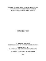
Figure 1.1: An example of mono-chromatic RkNN query.
Definition 1.1.6 (Mono-chromatic Reverse k-Nearest Neighbor Query) Given a dataset
S, query object q, a positive integer k and a distance metric Dist( ), mono-chromatic
reverse k-nearest neighbor query, denoted as RkNN(q, S), retrieves all objects p in S
such that Dist(p, q) ≤ Dist(p, q

), for ∀ q

∈ kNN(p, S), where kNN(p, S) are the
k-nearest neighbors of point p in dataset S.
RkNN(q, S) = {p|p ∈ SDist(p, q ) ≤ Dist(p, q

), ∀∧q

∈ kNN(p, S)}.

In the bi-chromatic case, the RkNN query has two input datasets - the point dataset
S and the query dataset R (also called site dataset in [115] ). The query dataset R is
different from the point dataset S. The query point q is from the site dataset R.
Definition 1.1.7 (Bi-chromatic Reverse k-Nearest Neighbor Query) Given a point
dataset S, a query dataset R, a query object q ∈ R, a positive integer k and a distance
metric Dist( ), bi-chromatic reverse k-nearest neighbor query, denoted as RkNN(q, R, S),
retrieves all objects p in S such that Dist(p, q) ≤ Dist(p, q

), for ∀ q

∈ kNN(p, R),
where kNN(p, R) are the k-nearest neighbors of point p in dataset R.
9
RkNN(q, R, S) = {p|p ∈ SDist(p, q) ≤ Dist(p, q

), ∀∧q

∈ kNN(p, R)}.
Figure 1.1 illustrates an example of the mono-chromatic RkNN query. Let dataset
S = {p
1
, p
2
, , p
8
}, p
2
be the query point and k=2. Since p
2
is one of the 2-nearest

neighbors of p
1
, p
3
and p
4
, R2NN(p
2
, S) = {p
1
, p
3
, p
4
}.
1.1.8 Classification of the Similarity Queries
Both the range query and the kNN query are classified as the basic similarity query
because of their comparatively low query cost. The naive solution to the range query
(the sequential scan method) scans the dataset S sequentially, computes the distance of
each object to the query object and then outputs the objects p such that Dist(p, q) ≤ r.
The naive solution to the kNN query maintains a sorted array of size k to store the k-
nearest neighbor candidates. Similarly, it scans the dataset S sequentially. When it finds
an object p that is closer to the query object q than the current k-th nearest neighbor
candidate, it inserts p into the sorted array and removes the current k-th nearest neighbor
from the candidates set. So both query is upper bounded by O(N) and can be solved
in O(N) time by scanning the point dataset S sequentially. N is the cardinality of point
dataset S. By utilizing the index techniques which will be introduced in Chapter 2, the
complexity of both queries can be reduced to O(logN) [16].
The range join and the kNN join are much more expensive than their single query
counterparts. Naive approach to answer a range join or a kNN join performs the range

query or the kNN query for each point in the query set R. This involves M (M is the
cardinality of R) times scanning of the dataset S, which introduces tremendous distance
computation and disk accesses. The query complexity of both the range join and the
kNN join is upper-bounded by the O(NM), where N is the cardinality of S and M is
the cardinality of R. For the self range join or the self kNN join, their query complexity
is upper-bounded by the O(N
2
), where N is the cardinality of S. Therefore, both queries
10
are categorized as the advanced similarity query.
Although the RkNN query only has one query point, it is also categorized as the
advanced similarity query because of its high computation complexity. Note that the k-
nearest-neighbor relation is not symmetric, that is, if p is one of q’s k-nearest neighbors,
q is not necessary to be one of p’s k-nearest neighbors. Therefore, the RkNN query is
much more complex than the kNN query. The naive solution for RkNN search has to
first compute the k-nearest neighbors for each point p in the dataset S (for the mono-
chromatic RkNN query) or R (for the bi-chromatic RkNN query). Then points p whose
distance from the query point Dist(p, q) is equal or less than the distance between p
and its k-th nearest neighbor can be determined as q’s reverse k-nearest neighbors. The
complexity of the first step is equal to the kNN join, so the complexity is upper-bounded
by O(N
2
) for mono-chromatic case and O(NM) for the bi-chromatic case. The second
step is a sequential scan of the dataset S. Therefore, it is also categorized as the advanced
similarity query.
1.2 Motivation
In the section, we describe the interesting applications of the kNN join, the RkNN query
and a specially property of the number of a point’s reverse k-nearest neighbors, which
motivated our research.
1.2.1 Motivation of the Study of the kNN Join

The kNN-join, with its set-oriented nature, can be used to efficiently support many im-
portant data mining tasks which have wide applications. In particular, it is identified that
many standard algorithms in almost all stages of knowledge discovery process can be
accelerated by including the kNN join as a primitive operation. For examples,
11
• Outlier analysis. Outlier analysis is to find out data objects that do not comply
with the general behavior or model of the data [52]. It has important applica-
tions such as the fraud detection (detecting malicious use of credit card or mobile
phone), customized marketing (identifying the spending behavior of customers
with extremely low or extremely high incomes) or medical analysis (finding un-
usual responses to various medical treatments) [52]. In the first step of LOF [23](a
density-based outlier detection method), the k-nearest neighbors for every point in
the input dataset are materialized. This can be achieved by a single self kNN-join
of the dataset.
• Data Classification. Data classification predicts the new data objects’ categorical
labels according to the model built according to a set of objects with known cate-
gorical labels (the training set). The knowledge of the new objects’ category can
be used for making intelligent business decisions. For example, it can be used to
analyze the bank loan applicants to identify the loan is either safe or risky. It also
can be used in the medical expert system to diagnose the patients. The k-nearest
neighbor classifier is one of the simplest but effective classification methods which
identifies the new object’s category by examining that object’s k-nearest neighbors
in the training set. The unknown sample is assigned the most common class among
its k-nearest neighbors. Given a set of unlabelled objects (the testing set), the kNN
join can be used to classify them efficiently by joining the testing set with the
training set.
• Data Clustering. Clustering is the process of grouping a set of physical or ab-
stract objects into classes of similar objects so that important data distribution
patterns and interesting correlations among data attributes can be identified [52].
It is also known as the unsupervised learning and has wide applications such as

pattern recognition, image processing, market or customer analysis and biological
12
research. The kNN join can be used in many clustering algorithms to accelerate
the process.
In each iteration of the well-known k-means clustering process [54], the nearest
cluster centroid is computed for each data point. A data point is assigned to the
its new nearest cluster if the previously assigned cluster centroid is different from
the currently computed one. A kNN join with k = 1 between the data points and
the cluster centroids can thus be applied to find all the nearest centroid for all data
points in one operation.
In the hierarchical clustering method called Chameleon [72], a kNN-graph (a
graph linking each point of a dataset to its k-nearest neighbors) is constructed
before the partitioning algorithm is applied to generate clusters. The kNN-join can
also be used to generate the kNN-graph.
Compared to the traditional point-at-a-time approach that computes the k-nearest
neighbors for all data points one by one, the set oriented kNN join can accelerate the
computation dramatically [19].
However, after the kNN join has been proposed recently in [20], to the best of our
knowledge, the MuX kNN join [20, 19] is the only algorithm that has been specifically
designed for the kNN-join. The MuX kNN join algorithm is an index-based join algo-
rithm and MuX [21] is essentially an R-tree based method. Therefore, it suffers as an
R-tree based join algorithm. First, like the R-tree, its performance is expected to degen-
erate with the increase of data dimensionality. Second, the memory overhead of the MuX
index structure is high for large high-dimensional data due to the space requirement of
high-dimensional minimum bounding boxes. Both constraints restrict the scalability of
the MuX kNN-join method in terms of dimensionality and data size.
As a consequence, new algorithms for efficient support of the kNN join in high-
dimensional spaces are highly desired. In this thesis, we design Gorder (the G-ordering