A behaviour based algorithm for encirclement of a dynamic target using multiple mobile robots
Bạn đang xem bản rút gọn của tài liệu. Xem và tải ngay bản đầy đủ của tài liệu tại đây (1.77 MB, 132 trang )
A BEHAVIOUR-BASED ALGORITHM FOR
ENCIRCLEMENT OF A DYNAMIC TARGET USING
MULTIPLE MOBILE ROBOTS
LOW YEE LEONG
(B.Eng.(Hons.), NUS)
A THESIS SUBMITTED
FOR THE DEGREE OF MASTER OF ENGINEERING
DEPARTMENT OF MECHANICAL ENGINEERING
NATIONAL UNIVERSITY OF SINGAPORE
2004
i
ACKNOWLEDGEMENTS
I would like to thank my supervisor, A/P Gerard Leng Siew Bing, for his intellectual
guidance and criticism, continuous support and understanding throughout my research
and study.
I would also like to thank my colleagues in Cooperative Systems Lab, especially Mr.
Cheng Chee Kong and Mr. Ng Wee Kiat for their help and interaction.
I am also thankful to staff in Dynamics Lab like Ms. Priscilla, Ms. Amy, Mr. Cheng,
and Mr. Ahmad for their assistance.
Last but not least, I would like to thank my family for their encouragement and
support. Without the love and backing from all of you, I would not be able to finish
the research.
ii
TABLE OF CONTENTS
ACKNOWLEDGEMENTS I
TABLE OF CONTENTS II
SUMMARY V
LIST OF TABLES VII
LIST OF FIGURES VIII
1 PROJECT DEFINITION 1
1.1 Problem Definitions and Assumptions 1
1.2 Definitions 2
1.2.1 Target 2
1.2.2 Encirclement 2
1.3 Thesis Outline 3
2 LITERATURE SURVEY 5
2.1 Circle Formation of Distributed Mobile Robots 5
2.2 Behaviour-Based Control of Multiple Robots 7
2.3 Chapter Summary 9
3 DESIGN OF ROBOTIC BEHAVIOURS FOR ENCIRCLEMENT 10
3.1 Three Basic Robotic Behaviours 10
3.1.1 Obstacle-Avoidance 10
3.1.2 Target-Tracking 11
3.1.3 Target-Circumnavigation 11
3.2 Robot Controller 13
iii
3.3 Behaviour Coordination 16
3.4 Encirclement Strategy 17
3.5 Chapter Summary 17
4 VALIDATION OF ENCIRCLEMENT ALGORITHM VIA SIMULATION 20
4.1 Program Structure 20
4.2 Implementation of Robotic Behaviours on Simulation 22
4.2.1 Obstacle-Avoidance 22
4.2.2 Target-Tracking 22
4.2.3 Target-Circumnavigation 22
4.3 Process of Encirclement on Simulation 25
4.4 Simulation Experimental Setup 27
4.5 Analysis of Simulation Results 28
4.5.1 Definition of Non-Dimensional Performance Index 28
4.5.2 Effects of Parameters on Performance Index 29
4.6 General Law for Performance Index of Encirclement 34
4.7 Chapter Summary 36
5 VALIDATION OF ENCIRCLEMENT ALGORITHM VIA HARDWARE
EXPERIMENTS 37
5.1 Robot Features 37
5.1.1 Obstacle-Detection Sensor 38
5.1.2 Target-Detection Sensor 40
5.1.3 Processor 41
5.2 Test of Individual Robot Behaviours 43
5.2.1 Obstacle-Avoidance 43
5.2.2 Target-Tracking 44
iv
5.2.3 Target-Circumnavigation 46
5.3 Hardware Experimental Setup 47
5.4 Comparison of Hardware and Simulation Results 49
5.5 Chapter Summary 49
6 CONCLUSIONS 52
6.1 Thesis Conclusions 52
6.2 Recommendations for Future Work 53
7 REFERENCES 54
8 APPENDICES 57
8.1 Simulation Results (Chapter 4) 58
8.2 Hardware Implementation Results (Chapter 5) 121
v
SUMMARY
The objective of this project is to formulate an algorithm that will coordinate the
movement of multiple mobile robots to encircle a dynamic target. The robots are not
equipped with global coordinate system and communication system. In addition, we
will study the performance of this algorithm for different number of robots used and
for different speed ratio (target speed / robot speed). Part of the results of this project
has been presented in the 2004 IEEE/RSJ International Conference on Intelligent
Robots and Systems (IROS) held in Japan.
In order to realize the algorithm, we have formulated three different reactive
behaviours for all the robots. The first behaviour is obstacle-avoidance, which makes
sure that a robot will not collide with obstacle. The second behaviour is target-
tracking, which guides a robot towards the target. The third behaviour is target-
circumnavigation, which leads a robot to move around the target. By adopting
subsumption-based coordination, a robot will execute one of these behaviours at any
one time according to the priority of the behaviour. Obstacle-avoidance has the
highest priority followed by target-circumnavigation and target-tracking. We have
also designed a simple neural controller to execute all these three behaviours.
We have implemented our algorithm on an object-oriented simulation C++ program.
Multiple simulations were performed to find out how the time taken changed for
different number of robots used and for different speed ratio. A general law governing
the performance and speed ratio of our algorithm was deduced from the simulation
vi
results. The performance is quantified by a non-dimensional index. We can use this
general law to predict the performance of the encirclement experiment as long as we
know the speed ratio regardless of the size of operational area, the speed of robots or
the speed of target.
We have also validated our algorithm by implementing it on physical robots that we
built. These robots have been used to perform encirclement experiments to validate
the feasibility of the simulation program. The results obtained from hardware
experiments agree with the simulation. Thus, we can use the general law deduced
from simulation to extrapolate the performance of hardware experiments.
vii
LIST OF TABLES
Table 3.1: Different sets of weights for different robot behaviours…………….16
Table 4.1: Relationship between speed ratio, target speed, and robot speed……28
viii
LIST OF FIGURES
Figure 1.1: Definition of encirclement. Highlighted sensors detect the robot within
the preset distance or the radius of encirclement…………………… 3
Figure 2.1: Reuleaux’s triangle……………………………………………………6
Figure 2.2: Motor schema architecture……………………………………………8
Figure 2.3: Example of subsumption architecture……………………………… 9
Figure 3.1: Basic behaviour 1: Obstacle-avoidance…………………………… 11
Figure 3.2: Basic behaviour 2: Target-tracking………………………………… 12
Figure 3.3: Basic behaviour 3: Target-circumnavigation……………………… 12
Figure 3.4: Network structure of the robot controller…………………………….14
Figure 3.5: Relationship between weights numbering and robot’s directions……15
Figure 3.6: Subsumption-based coordination of behaviours…………………… 16
Figure 3.7: Switching between target-tracking behaviour and target-
circumnavigation behaviour………………………………………….18
Figure 3.8: Obstacle-avoidance behaviour makes robots distribute more evenly
around the target…………………………………………………… 19
Figure 4.1: Class structure of simulation program……………………………… 21
Figure 4.2: Implementation of (a) obstacle-avoidance and (b) target-tracking on
simulation. Robot’s direction is indicated by the white arrow on the
robot body…………………………………………………………….23
Figure 4.3: Implementation of target-circumnavigation on simulation. Robot’s
direction is indicated by the white arrow on the robot body…………24
Figure 4.4: Selected images of the encirclement simulation: (a) the initial
distribution, (b) – (e) intermediate steps, and (f) completion of
encirclement………………………………………………………….26
Figure 4.5: Graph of the non-dimensional performance index versus speed
ratio………………………………………………………………… 30
ix
Figure 4.6: Graph of non-dimensional performance index versus number of
robots…………………………………………………………………31
Figure 4.7: Graph of success rate versus speed ratio…………………………… 32
Figure 4.8: Maximum speed ratio for encirclement. R can be considered as the
radius of encirclement……………………………………………… 33
Figure 4.9: Graph of non-dimensional performance index vs smaller speed
ratio………………………………………………………………… 34
Figure 4.10: Graph of log(non-dimensional performance index) vs log(speed
ratio)………………………………………………………………….35
Figure 5.1: Devantech SRF08 Ultrasonic Ranger……………………………… 38
Figure 5.2: Field of view of SRF08 Ultrasonic Ranger. (From the website of the
manufacturer, [16])…………………… 39
Figure 5.3: Calibration graph of sonar sensor couple in Devantech SRF08
Ultrasonic Ranger…………………………………………………….39
Figure 5.4: Calibration graph of light sensor coupled in Devantech SRF08
Ultrasonic Ranger…………………………………………………….40
Figure 5.5: Microcontroller used: Acroname BrainStem GP 1.0……………… 41
Figure 5.6: A photograph of the robot. It becomes a target when a light bulb is
mounted on it…………………………………………………………42
Figure 5.7: Robots displaying obstacle-avoidance behaviour……………………44
Figure 5.8: Robots displaying target-tracking behaviour……………………… 45
Figure 5.9: Robot displaying target-circumnavigation behaviour……………… 46
Figure 5.10: Snapshots of hardware experiment………………………………… 48
Figure 5.11: Comparison of hardware and simulation results. (Speed Ratio: 0.2) 50
Figure 5.12: Comparison of hardware and simulation results. (Speed Ratio: 0.3) 50
Figure 5.13: Comparison of hardware and simulation results. (Speed Ratio: 0.4) 51
1
Chapter 1
PROJECT DEFINITION
The problem of encirclement of a dynamic target is very common in real life
applications. For example, the policemen will try to chase, encircle and finally arrest
the criminals when they are executing the operation. The soldiers will try to encircle
and capture the enemy during the war. In rugby games, the players will try to encircle
and catch their opponents. During the process of encirclement, some parameters are
critical to the overall performance of the results like the number of pursuer/hunter and
the speed ratio of the pursuer/hunter to the target. In this project, we will replicate the
encirclement problem using multiple mobile robots in simulation and hardware
experiments. We will develop an algorithm for multiple mobile robots to encircle a
dynamic target and finally find out the relationship between the important parameters.
1.1 Problem Definitions and Assumptions
The main challenge of this project is to formulate an algorithm to encircle a target
using multiple mobile robots from random initial positions. In order to define the
problem more precisely, we have made the following assumptions:
1. The target is dynamic and it will try to escape from the encirclement of the
robots when obstacle-avoidance behaviour of the target is triggered.
2
2. The target is initially located within the sensor range of the robots. That means
the robots know where is the target when the experiment starts. The robots
need not spend extra time to search for the target.
3. The environment for the robots to move is a flat ground without obstacles.
Each robot is free to move on the ground unless the distance to the nearest
robot or target is small enough to trigger the obstacle-avoidance behaviour.
4. The robots are moving at the same speed so that the speed ratio (target speed /
robot speed) is common for all robots in experiment. This will help us to
investigate the effect of speed ratio on the performance.
5. The robots are not equipped with global coordinate system and
communication system. Each robot must be able to encircle the target based
on its own sensor readings.
1.2 Definitions
1.2.1 Target
The target used in our project is a light bulb on top of a robot. There are two types of
target used in experiment, i.e. stationary and dynamic. Stationary target means that the
robot carrying the light bulb is not moving while dynamic target is mounted on a
moving robot. The robot can avoid other robots when it is moving in the environment.
1.2.2 Encirclement
3
Encirclement takes place when the robots are distributed in the four quadrants of the
target. They need not to be at equal distance from the target so long as the distance
between the robot and the target is smaller than a preset value. This value can be
treated as the radius of the encirclement. Figure1.1 illustrates the definition of
encirclement.
1.3 Thesis Outline
The contents of all chapters are summarized below.
Chapter 2 surveys related research works related to the encirclement problem. These
works are divided into two sections: circle formation of distributed mobile robots and
behaviour-based control of multiple robots.
Chapter 3 will first introduce the three basic robotic behaviours used in our project.
These three behaviours are obstacle-avoidance, target-tracking, and target-
circumnavigation. Then we will describe the robot controller we have designed to
Figure 1.1
Definition of encirclement. Highlighted sensors detect the robot within the preset distance
or the radius of encirclement.
4
execute the robotic behaviours. After that, we will present an architecture that can
coordinate the three behaviours in such a way that an encirclement of target will be
completed.
Chapter 4 validates the encirclement algorithm via a simulation program we have
written. The individual robotic behaviour and the process of encirclement
implemented on simulation are shown here using snapshots of the program. After
discussing the experimental setup, we will analyse the simulation results by using a
non-dimensional performance index. A general law governing the performance and
the speed ratio (target speed / robot speed) of our encirclement algorithm will be
given.
Chapter 5 discusses the implementation of our encirclement strategy onto our own
physical robots. A description of the physical robot will be given and the performance
of the robots will be presented as well.
Chapter 6 gives a conclusion of this project and provides some recommendations for
future work.
5
Chapter 2
LITERATURE SURVEY
This chapter will give a survey of research work related to the encirclement problem.
They are divided into two parts: circle formation of distributed mobile robots and
behaviour-based control of multiple robots.
2.1 Circle Formation of Distributed Mobile Robots
Coordinated movement is a common phenomenon in nature, e.g. wolves hunt in a
pack to increase their success in capturing prey. Animals can benefit from coordinated
movement by combining individual sensing ability. In the robotics world, coordinated
movement or formation control is also a major research topic. Research in this area
can be found in reference [1] to [8].
The encirclement problem originated from the circle formation problem, which has
been a very interesting problem in this research area of distributed mobile robotics.
The best-known solution is the distributed algorithm proposed by Sugihara and
Suzuki [1,2]. In this algorithm, each robot is represented by a point and able to move
in any direction. In addition, this algorithm requires each robot to know the distance
to its farthest (D
i
) and nearest (d
i
) neighbours, respectively without the aid of a
centralized coordinator. After the farthest and nearest distances are known, the
algorithm tries to match the ratio of D
i
/ d
i
to a prescribed constant. Therefore, the
6
algorithm requires each of the robots to know the positions of all other robots. In
order to achieve this requirement in practice, a perfect sensor that can enable the robot
to “see” the location of all other robots is needed. This algorithm seems workable in
simulation. A simulation program has been written to verify this algorithm. But, as
reported in their paper, sometimes a shape of constant diameter like a Reuleaux
triangle (see Figure 2.1) rather than a circle is formed. In a Reuleaux triangle, arcs ab,
bc and ca are drawn with radii equal to D, from the vertices c, a and b. Triangle abc is
also an equilateral triangle with sides equal to D.
In another study, Yun, Alptekin, and Albayrak have proposed an algorithm for robots
to form a circle under limited sonar range [3]. For this algorithm, the initial positions
of robots are randomly placed in a large rectangular field. The field is so large that a
robot may not see other robots due to limited sonar sensor range. In order to make the
robots form a circle in a large field, all the robots need to converge to the centre of the
field first. Therefore, this algorithm is not applicable to field of other shapes because
it requires the robot to record the coordinates of the first and third corners of the field
while following along the edges so that it can converge to the centre of the rectangular
field. Similar to [1,2], this algorithm is only demonstrated in simulation rather than
Figure 2.1
Reuleaux’s triangle.
a
c
b
D
D
D
7
real robot implementation. A global coordinate system is also needed for the robots to
find out where is the centre of the rectangular field.
Fredslund and Mataric have suggested a general algorithm for robot formations using
local sensing and minimal communication [4]. Thus, no global positioning system is
required. In their algorithm, the robots are provided with information of the total
number of participating robots. A conductor/leader robot that will then decide on the
type and the heading of the formation while the rest of the robots need only to keep a
certain distance and angle to their neighbours. With this approach, communication has
been kept to the minimal.
2.2 Behaviour-Based Control of Multiple Robots
Robots are usually equipped with different kind of sensors to interact with the
environment. The robots will exhibit different behaviours depending on how the
sensor is connected to the motor. Braitenberg [9] is one of the earliest scientists who
studied this topic. He has designed some vehicles that used inhibitory and excitatory
influences directly coupling the sensors to the motors. Some seemingly complex
behaviours like cowardice, aggression, and love can result from relatively simple
connection between sensors and motors.
Global robot formation can be emerged from multiple robots undergoing behaviour-
based control. In a behaviour-based control system, a robotic architecture is used to
coordinate the robotic behaviours. One of the common architectures is called motor
schemas architecture, developed by Ronald Arkin [10-12]. Figure 2.2 shows a typical
motor schema architecture. Each motor schema has an action vector that defines the
way the robot should move in response to the perceived stimuli. These responses are
8
generated using potential field approach. Different behaviour will output different
motor schema. The coordination between these different motor schemas is done by
vector addition. Each behaviour can contribute in varying degrees to the robot’s
overall response by setting different gain. In [8], Balch and Arkin have shown that
formation behaviour can be integrated into a motor-schema behaviour-based system
with other navigational behaviours so that a robotic team can reach navigational goal,
avoid hazards and simultaneously maintain in their intended formation.
The other common architecture for behaviour-based robotic control system is called
subsumption architecture. This architecture was developed by Rodney Brooks [13]. It
is a purely reactive behaviour-based and layered control system. Figure 2.3 shows one
of the examples of subsumption architecture. Priority-based arbitration is the
coordination mechanism, and the robot is executing only one behavioural rule at any
time. In this example, homing behaviour has the highest priority while wandering is
the least important behaviour. We are using this architecture because we find that it is
easy to implement on our robots.
Sensors
S
1
S
2
Motor Schemas
MS
1
MS
2
Vector
Σ
Motors
Figure 2.2
Motor schema architecture.
9
2.3 Chapter Summary
We have discussed the related research works in the fields of circle formation of
distributed mobile robots and behaviour-based control of multiple robots. Inspired by
[1] and [2], our work studied the encirclement problem of a target. Instead of global
knowledge of other robots’ positions, our robots use only local sensing and do not
share a common coordinate system, as in [4]. In contrast to this work, our approach is
completely independent of any explicit forms of communications. We also use
behaviour-based control system to coordinate the movements of robots like [8] but we
use subsumption architecture instead of motor-schema architecture.
Figure 2.3
Example of subsumption architecture.
Homing
Pickup
Avoiding
Wandering
S
S
S
S
: Suppress
10
Chapter 3
DESIGN OF ROBOTIC
BEHAVIOURS FOR
ENCIRCLEMENT
This chapter will first discuss the three basic robotic behaviours we have designed for
encirclement. These three behaviours are obstacle-avoidance, target-tracking, and
target-circumnavigation respectively. After that, we give introduce a neural controller
we have designed to execute the required robotic behaviours. Finally, how the
coordination of the behaviours can achieve encirclement will be explained.
3.1 Three Basic Robotic Behaviours
3.1.1 Obstacle-Avoidance
When an obstacle, which can be other robot or the target, is detected by any of the
sonar sensors, (i.e., the sonar sensor reading is below a certain threshold value, T
S
),
the robot should stop first, turn to the opposite direction from the obstacle, and then
move forward (see Figure 3.1). Therefore, a change of direction is required. For
example, with reference to Figure 3.1, if the right sensor detects an obstacle, the robot
should stop the forward motion first, and then rotate 180 degrees so that the robot
heads in the direction of the left sensor before it starts to move forward again.
11
3.1.2 Target-Tracking
We have assumed that the target is initially located within the light sensor range of the
robots. Therefore, when the experiment starts, the robots should turn toward the target
and move forward (see Figure 3.2). In this case, change of direction is required also.
By taking the example in Figure 3.2, when the target is located at the upper-right
sector of the robot’s precinct, the light sensor reading at that sector will be big enough
to overcome the first light threshold, T
L1
. So, the robot should stop the forward
motion first, and then turn to the upper-right direction. After the turning motion is
finished, the robot should move forward again.
3.1.3 Target-Circumnavigation
When the robot moves closer to the target, the light sensor reading will increase at the
same time. Once the reading exceeds the second light threshold, T
L2
, the robot should
stop moving toward the target. It should now turn to either the left or the right
(depending which direction the robot wants to encircle the target; left is for clockwise
direction, right is for counter-clockwise direction) and move forward (see Figure 3.3).
Figure 3.1
Basic behaviour 1: Obstacle-avoidance.
Robot’s original direction
Robot’s new direction
12
For the case of counter-clockwise direction, when the light sensor reading exceeds the
second light threshold, the robot should stop the forward motion first, then turn to the
right. After the turning motion is finished, the robot should move forward again. For
this behaviour, change of direction is required also.
Target
Figure 3.2
Basic behaviour 2: Target-tracking.
Robot’s original direction
Robot’s new direction
Target
Robot’s original direction
Robot’s new direction
Figure 3.3
Basic behaviour 3: Target-circumnavigation.
13
3.2 Robot Controller
In order to execute a robotic behaviour, we must know how to process sensor
information and then give a corresponding output for the motor to achieve. Inspired
by a neural perceptron [17], we have designed a neural controller to execute the robot
behaviours. This neural controller can take input from all the eight sonar sensors and
eight light sensors positioned evenly at the circumference of the robot (see Figure
3.4). There are two different outputs from the perceptron. One of them is the angle for
the robot to turn, while the other is the signal to move forward.
Our controller is a simple, one-layer feed-forward neural network with eight input
nodes and two output nodes, whereby each of the input signals, x
i
, is either 1 or 0
depending on the sensor reading. For a sonar sensor, if its reading is smaller than a
certain threshold value, T
s
, the input signal will be set to 1; else, it will be set to 0. The
rule is reversed for light sensor. The input signals will then be multiplied by synaptic
weights, w
i
, which has a value between 0 and 1. The two output signals are the
outcomes computed from the functions of the sum of these eight weighted input
signals.
There are two different output functions. The first output is the angle for the robot to
turn. The relationship between the angle and the input signals is shown in Equation
(3.1).
Angular displacement,
360*
ii
xw
=
θ
(3.1)
Angular displacement θ is a vector with magnitude between 0 and 360 degree. Its
direction is pointing normally out of the plane. After turning with this angular
14
displacement θ, the robot will point to one of the headings of the eight sensors (see
Figure 3.5).
For the other output signal, v, when the sum of weighted inputs is zero or none of the
sensors is activated, v should be 1. And thus the robot should move forward at a
constant speed. It is expressed in Equation (3.2).
else
xwif
v
ii
0
0
1 =
=
(3.2)
Σ
Synaptic weights
Body of the robot
Sonar and light
sensors
8 sensor inputs, x
i
Σ
f
1
f
2
θ
v
Synaptic
weights, w
i
Output
functions
Figure 3.4
Network structure of the robot controller.
15
This controller is very useful for executing the robot behaviours requiring the robot to
change its direction. Different robot behaviour will have different sets of weights.
Which set of weights will be used depends on which behaviour is activated.
After knowing how the robot will react under three different situations, we can
summarise the synaptic weights in Table 3.1. The first weight is always connected to
the front sensor, followed by the next sensor in a counter-clockwise direction (see
Figure 3.5).
These weights are arrived at based on how much the angular displacement the robot
needs to execute for different behaviours. For example, if a robot wants to avoid an
obstacle at front, the required angular displacement should be 180°. The weight for
the front sensor should then be 0.5 so that w
0
* x
0
* 360° = 0.5 * 1 * 360° = 180°.
Right
Left
Front
Back
Figure 3.5
Relationship between weights numbering and robot’s directions.
Forward direction
w
0
w
1
w
2
w
3
w
4
w
5
w
6
w
7