Stochastic dominance in stock market 4

91
Chapter 4
The “New Economy” versus the “Old Economy”, which is preferred?

4.1 Introduction
From 1998 to the first quarter of 2000, investors were extremely optimistic about
Internet companies. They were mesmerized by the “dot-com” fad. Any company with
a .com in its name was rewarded with a high valuation. The quantum of investment
money and the number of company formations have “skyrocketed”, observed Bill
Gates (Perkins and Perkins 1999). Internet stocks became the new favorite on Wall
Street and hailed as the “new economy”. However, prosperity sustainable did not last
for long. Many investors as well as investment analysts, who had happily enjoyed the
great initial gains from Internet stocks for more than two years, were shocked by the
dramatic downturn in the spring of 2000. Since then, they have been jolted from the
dot-com sweet dream and started experiencing the painful truth of this new economy.

The prices of Internet stocks went up and down at more extreme volatile rates
than other conventional stocks between 1998 and 2000. Hence, investments in
Internet stocks are likely to either generate big wins or enormous losses. Looking at
the statistics, the NASDAQ 100 Index increased 140% compared to 33% in the S&P
500 Index from June 1998 to March 2000. After the peak on March 2000, NASDAQ
100 decreased 70% by the end of 2000 while S&P 500 only declined by 14%. In 1999,
the Dow Jones Industrial Average (DJIA) increased 20%, the NASDAQ was up 86%,
and Peter S. Cohan & Associates’ Internet Stock Index rose 339%. In 2000, however,

92
the Internet Stock Index had lost 67% of its value, while the DJIA depreciated 6% and
the NASDAQ fell 39%. Over the two years under analysis, Internet stocks rose by 6%,
the DJIA appreciated 18%, and the NASDAQ had gained 13% of its value (Cohan
2001). Demers and Lewellen (2003) reported that 294 Internet firms went public in

1999 and raised more than $20 billion in capital. By March 1, 2000, Internet firms had
a combined market value of $1.7 trillion. Between January 1999 and February 2000,
the Internet Stock Index more than tripled in value. However, by 2001, the industry
suffered a total decline of 90% (Lewellen 2003).

Academics and analysts started to question this dramatic rise and fall of
Internet stocks prices. What are the causes of this Internet bubble burst which
occurred within a two-year time period? Are new economy stocks overpriced? Is the
dramatic rise and fall of Internet stocks due to irrational investors’ behavior or insider
action? Will the risk-averse and risk-seeking investors have different preferences on
Internet stocks to maximize their utility?

Many studies have attempted to explain the downfall of Internet stocks
especially since the bubble burst in the spring of 2000. Although many studies have
examined misperceptions on Internet stocks, there is still a persistent lack of literature
on the comparisons between the old and new economy stocks. All the literature to
date uses individual companies as sample in their studies and none looked at the
market from a broader perspective to study the market indices. The downfall may be
attributed to investors’ behavioral or fundamental account variables, lack of broad
picture focus on the risk-based preference of investors. Hence, this study tries to fill
the gap mentioned here. The issue of market efficiency and rationality is not the key

93
point here as it has been widely discussed in the literature and the imperfect
knowledge of the current asset pricing benchmarks. The main objective of this study
is to investigate whether investors’ enthusiasm for Internet stocks is consistent with
utility maximization. A more general framework for analyzing utility choices,
stochastic dominance (SD), is used in this study. The findings of this study will hold
an important lesson for investors on how to deal with similar bubbles if they arise in
the future. In addition, the stocks preferences of different types of investors will also

be examined.

The empirical results show that neither S&P 500 nor NASDAQ 100
stochastically dominates each other at first order for the whole sample period and the
two sub-periods. Surprisingly, there is no evidence of the new economy dominance
even during the Internet boom. S&P 500 dominates at the left-hand (negative returns)
side while NASDAQ 100 dominates at the right-hand (positive returns) side. However,
S&P 500 stochastically dominates NASDAQ 100 at second order implies that risk-
averse investors prefer old economy stocks to new economy stocks. Furthermore,
evidence of old economy stocks dominance is generally stronger at third-order SD
than the second-order SD. This implies that investors who prefer more positive
skewness would also have chosen to buy old economy stocks only. These results
suggest that the Internet stocks would never be better than the old economy stocks for
the entire sample period. The evidence of old economy stocks dominating is even
stronger after the bubble burst. It is also found that risk lovers prefer new economy
stocks to old economy stocks while investors with S-shaped or reverse S-shaped
utility function have no preference between old and new economy stocks. Invertors

94
may use these findings as a reference for their investment decisions on old and new
economy stocks.

This chapter is organized as follows. Section 2 comprises of a literature review;
section 3 describes the SD methodology. Section 4 discusses the sample and data;
section 5 constructs the SD tests, section 6 reports the SD results, section 7 discusses
some special cases and section 8 concludes this chapter.

4.2 Literature Review
Several researchers have examined investors’ behavior when valuing the Internet
stocks. Cohan (2001) observes the manifestations of investor’s fear from the stock

indices. First, investors sell everything and put the earnings into the most rapidly
growing sectors because they fear of losing out on rapid growth. Panic selling and
drops in these rapidly growing sectors then lead the investors to put their money into
old economy stocks which they believe of preserving the gains they have made in the
fastest-growing sectors.

The relationship between the performance of Internet stocks and their peers is
very complex. When investors are afraid of falling behind, Internet stocks tend to go
up the most because investors feel that the Internet stocks are in the fastest-growing
sector of the economy. When investors are afraid of losing their gains, they tend to
sell the Internet stocks and invest their earnings in the old economy stocks that are
likely to hold their value better in a slowing economy. During these periods, the
Internet stocks tend to perform less well than their peers. (Cohan 2001)


95
Wheale and Amin (2003) explain the burst from the change of investors’
behavior on valuing the Internet stocks before and after the burst. Six measures,
namely, return on assets, return on equity, price-sales ratio, price-earnings ratio, book
value and free cash flow are selected as indicators of corporate performance. They
examine the relationship between stock returns and these six indicators before and
after the collapse. The evidence from their study suggests that only price-sales ratio,
price-earnings ratio, book value and free cash flow are value-relevant before the burst.
However, after the burst, all six indicators are value-relevant. Hence, they claim that
investors’ valuation on Internet stocks have changed from emphasizing on revenue to
profits. Therefore, they stress the importance of behavioral finance in classical
financial theory.

Ofek and Richardson (2003), however, hypothesize on heterogeneous
investors with short sales restrictions (via IPO) to explain the Internet bubble burst in

Spring 2000. They study various characteristics like volume, share turnover, short
interest, rebate rate etc. of Internet companies. From the beginning of 1998 to 2000,
there were many optimistic investors willing to pay high prices for the Internet stocks.
On the other hand, there were some pessimistic investors willing to short these stocks
at high prices. However, the short sales restrictions lead to the rises of Internet stocks
prices. During the spring and latter half of 2000, many lockups expired. Thus,
pessimistic investors and insider sales cause the Internet stocks prices to drop. In
addition, the holding of retail trader for Internet stocks more than institutional traders
shows heterogeneity among investors. Hence, the market is more prone to behavioral
biases. Moreover, retail day traders have driven momentum investing in recent years
(Perkins and Perkins 1999).

96

On the other hand, traditional accounting model does not carry sufficient
information about the growth opportunities and intellectual assets that may make up
major components of Internet firms’ values. Several researchers have studied
systematic relationships between stock prices, accounting variables and non-financial
measures of resources and performance (see Trueman, Wong and Zhang 2000,
Rajgopal, Venkatachalam, Kotha and Erickson 2002). In addition, there are
widespread claims that stocks in this sector were overpriced in 1999, and other
researchers (for example, Demers and Lev 2001) have investigated the factors
associated with the Internet “pricing shakeout” in early 2000, with a focus on non-
financial value drivers. Existing Internet valuation studies find mixed results when
examining the relation between traditional financial measures and market values of
Internet firms during 1999 and early 2000. Their results provide some support for the
importance of cash availability for Internet firms, particularly after the downturn in
Spring 2000 (Keating, Lys and Magee 2003).

Jahnke (2000) discusses new approaches like top-line revenue growth,

customer growth, website visits, peer group comparison and momentum to value
Internet stocks. He points out that the new economy stocks are overpriced. The price
being set by investors to play the Internet revolution is too high relative to the profits
the industry is likely to produce in the future. Investors have wrongly assumed that
glamour-investing produces superior investment returns. He reminds the investors that
great technological innovation do not necessarily translate into great investment
opportunities for the typical investor. Producing high rates of revenue and earning

97
growth rates over many years is rare. As companies get bigger, it becomes harder to
grow at above average rates.

King (2000) suggests that the best way to value a single e-business company is
to apply traditional valuation methodologies. Follow the usual approach of valuation,
first, the present value of the future cash flows is determined. Then, the projected cash
flows are discounted at an appropriate discount rate. An indication of the value for an
e-business company is the sum of these discounted amounts.

Keating, Lys and Magee (2003) show that traditional financial variables and
new economy measures can explain much of the cross-sectional variation in prices
and returns of Internet stocks in the spring of 2000. However, Lewellen (2003) argues
that their results tell more on investor’s irrationality or misperception than as
suggested by them on the agency cost and information asymmetries. This irrational
view suggests why prices rise so dramatically in the first place.

Besides investors’ behavior and stock valuation methods, there is literature
focus on IPO underpricing in investigating the Internet bubble. There is widespread
belief among both academics and practitioners that the prices of Internet IPO cannot
be justified by economic fundamentals. Managers and bankers are taking the
advantage of irrationally high prices to sell Internet stocks. Ritter (1991), Loughran

and Ritter (1995) and many others show that Internet IPOs significantly underperform
as compared to other stocks of similar size in the same industry for five years after
going public.


98
According to Perkins and Perkins (1999), as capital begins to flood the market,
companies not only start up faster but also go public sooner. A financial food chain
includes the entrepreneurs, the venture capitalists, the investment bankers and certain
large institutional investors and mutual funds play an important role in IPO. In the
Internet boom era, venture capitalists are pushed by both their investors and
entrepreneurs they invest in to shoot quickly for an IPO. On the other hand, the
investment banks willing to serve their investors for Internet IPO so they can collect
their 7% underwriting fees and engage new clients to manage their follow-on
offerings. At the end, companies that shouldn’t be public are public.

Perkins and Perkins (1999) also state that narrow float which means the
limited number of company shares available to public investors drive up the Internet
stocks prices. When demand is high and the supply is limited, the prices of these
stocks skyrocket. Furthermore, insiders keep more of the stocks from their Internet
startups for themselves. In the first half of 1998, these companies offered only 31% of
their total capitalization to public investors. This allows them to sell their stocks at a
greater profit following the significant share appreciation typical in bubble markets.

Schultz and Zaman (2001) find that the Internet firms sell smaller proportion
of their equity and insiders sell fewer of their own shares in the IPO. This implies that
insiders expect prices to remain high for a long time and therefore there is no hurry to
sell or they feel the IPOs are underpriced and prefer to sell later.

Ljungqvist and Wilhelm (2003) suggest that the unique characteristics on

ownership structure and insider selling behavior of firm during the “dot-com bubble”

99
cause the IPO underpricing. The decline of CEO, venture capitalists and investment
banks stakes cause the ownership to be more fragmented. These changes of ownership
then cause the secondary sales to decrease sharply.

How true does the media hype sharing market gossip via Internet impact on
the Internet stocks prices? Demers and Lewellen (2003) explore the potential
marketing benefits of going public and IPO underpricing. Internet companies
experience high publicity surrounding their IPO. They suggest that the marketing
benefits of underpricing extend beyond the Internet sector and the “hot issues” market
in the late 1990s. If underpricing attracts media attention and creates valuable
publicity for issuing firms, this effect should be reflected in an increased number of
website visitors following the IPO.

Beneath the surface of the statistics, there are unique activities that drive the
movement of money in and out of Internet stocks. Day traders, message boards,
influential analysts and the pervasive influence of the cable-TV network CNBC all
have a real impact on the day-to-day flow of money in the markets. In some cases,
these money drivers are simply new technologies that have speeded up the traditional
process of sharing market gossip. In other cases, these phenomena are new and
surprisingly powerful (Cohan 2001).

Grodinsky (1953) points out that when new industries are born, there often is a
rush by many companies to enter the field in this period of initial and rapid growth.
This is followed by a shakeout period with only a relatively few survivors and by a
continuing period of strong growth, although the rate of growth is slower than the

100

initial period. Finally, industries are expected to stop growing, either living a
relatively stable existence for an extended period of time or dying. Grodinsky points
out the great risk of selecting stocks in the pioneering stage, where little information
about participants may be available. There is little or no past record to guide investors
or aid them in preparing future projections.

Any new industry will follow the four stages of industry life cycle. Internet
companies are in the start-up stage. In the long run, this new industry will develop and
mature to become old economy and everything will return to normal. Although many
have suffered from the Internet bubble burst, Koller (2001) advises that investors
shouldn’t abandon the Internet stocks. Nevertheless, they should understand the basic
principles of value creation and generate new insights into the potential value of
Internet opportunities. Investors should look forward to a better tomorrow.

All the literature above try to explain the downfall of Internet stocks attributed
to investor’s behavior, accounting methods, IPO underpricing etc. while this study
contributes to the literature by looking at different direction that is investor’s utility
maximization.

4.3 Stochastic Dominance
The SD approach is used to examine whether the new economy stocks dominates the
old economy stocks or vice versa in this study. The SD approach provides a general
framework for studying economic behavior under uncertainty. Hadar and Russell
(1969), Hanoch and Levy (1969), Rothschild and Stiglitz (1970), Whitmore (1970)
lay the foundation of SD analysis. Levy (1992, 1998) provides an up-to-date summary

101
of SD and its applications in economics and finance. In finance, the SD approach has
been used to study option pricing (Levy 1985), the small-firm effect (Seyhun 1993),
portfolio selection (Post 2003) and momentum effect (Fong, Lean and Wong 2004).

Up to my knowledge, I believe this is the first study that uses SD approach to study
Internet stocks.

Suppose there are two assets, X and Y, the probability of exceeding any return
in X is always at least as high as in Y. For a non-satiation investor, he will prefer asset
X to asset Y. An investment decision can be made without having the particular
mathematical form of investor’s utility function. SD is generally described by the
determination of an order of preference between two assets. It is not dependent on
distributional assumptions and risk measures. For case here, X can be referring to the
returns of the new economy stocks with cumulative distribution function (CDF)
F

and Y refers to the returns of the old economy stocks with CDF
G . Assuming that
investors prefer more to less, an investor who want to maximize his expected utility
would prefer
F which lies below
G
. Chances to earn higher returns are always
greater with
X than Y; regardless the investor likes or dislikes risk. More explanation
of SD can be found in the previous chapters.

4.4 Sample and Data
S&P 500 and NASDAQ 100
1
are used to represent the old and new economy stocks
respectively. S&P 500 can be called “old economy stocks index” or simply the “old
stocks” and NASDAQ 100 can be called “new economy stocks index” or simply the

1
CRSP and @Net Index have also been examined as proxies to old and new economy stocks. As the
results are similar, only the results for S&P 500 and NASDAQ 100 are reported in this chapter.

102
“new stocks”. The NASDAQ 100 Index includes 100 of the largest domestic and
international non-financial companies listed on The NASDAQ Stock Market based on
market capitalization. The index reflects companies across major industry groups
including computer hardware and software, telecommunications, retail/wholesale
trade and biotechnology. It does not contain financial companies including investment
companies. Both daily indices are obtained from Datastream.

With the assumption that the history is likely to repeat by itself in the future
and hence analyze the past will help us to make inference for the future. The sample
for this study covers the period from January 1998 to December 2003. The sample
period starts from 1998 because there is a clear upward trend for Internet stocks
around this period. This sample period spans a period of intense IPO and secondary
market activities for Internet stocks. The sample is further divided into two sub-
periods to look at the effect of bubble burst. The first sub-period is a bull run for
Internet stocks from 1 January 1998 to 9 March 2000 (before crash) and the second
sub-period is a bear market for Internet stocks from 10 March 2000 to 31 December
2003 (after crash). For simplicity, the first sub-period is called “bull sub-period” and
the second sub-period is called “bear sub-period”.

4.4.1 Preliminary Analysis
Table 4.1 reports daily returns of NASDAQ 100 and S&P 500 for the whole sample
period and two sub-periods.

For the whole sample period, mean returns are positive for both S&P 500 and

NASDAQ 100. The mean daily returns are 0.01% for S&P 500 and 0.03% for

103
NASDAQ 100 which translate to annualized returns of 2.6% and 7.8% respectively.
The mean returns for NASDAQ 100 is three times higher than S&P 500 for whole
sample period. Hence, by using means alone, everybody will prefer to long new
stocks.


Table 4.1: Descriptive Statistics of Daily Returns for Indices in
Whole Sample Period and Two Sub-Periods

S&P 500 NASDAQ 100
Whole Period
mean 0.0001 0.0003
t-stat 0.26 0.38
median 0.0000 0.0007
standard deviation 0.0130 0.0265
skewness 0.0102 0.1695
kurtosis 1.8775 2.2157
correlation 0.8342
Bull Sub-Period
mean 0.0006 0.0027
t-stat 1.27 3.02
*

median 0.0005 0.0035
standard deviation 0.0122 0.0212
skewness -0.3809 -0.3706
kurtosis 2.7596 1.1470

correlation 0.8308
Bear Sub-Period
mean -0.0002 -0.0011
t-stat -0.54 -1.25
median 0.0000 0.0000
standard deviation 0.0135 0.0289
skewness 0.1871 0.3544
kurtosis 1.5447 2.1204
correlation 0.8405
Note: * significant at 1% level.


However, when we look at each sub-period, a different conclusion is drawn:
investors will prefer new stocks in the bull sub-period and prefer old stocks in the
bear sub-period. Compared to the old stocks, new stocks go up more in the bull

104
market and down more in the bear market. Before crash, the annual mean returns are
15.6% for S&P 500 and 70.2% for NASDAQ 100 which is nearly five times higher. It
seems the returns of new stocks are too high while the returns of old stocks are too
low during the two-year’s market boom. However, after crash, the annual mean
returns are -5.2% for S&P 500 and -28.6% for NASDAQ 100 which is more than five
times lower than S&P 500! This implies that the new economy stocks generate big
wins and enormous losses within a short period of two years. This divergence
between the old and new stocks suggests that investors tend to put their money into
the new stocks when they are afraid of losing out on growth opportunities and they
scramble into old stocks when they fear a drop as they want to preserve the gains they
made in their new stocks (Cohan 2001).

Mean-variance criterion uses both “mean” and “variance” (or “standard

deviation”) together to make inference. It is well-known that risk averters prefer stock
with higher mean and smaller variance while risk lovers prefer stock with higher
mean and higher variance. As the means are 0.03% and 0.01% and the standard
deviations are 2.65% and 1.3% for the new and old stocks respectively, risk averters
have no preference between the old and new stocks while risk lovers prefer new to old
stocks in the whole period. One will draw the same conclusion in the bull sub-period.
However, in the bear sub-period, the means are -0.11% and -0.02% and the standard
deviations are 2.89% and 1.35% for the new and old stocks respectively. Hence, risk
averters prefer old stocks while risk lovers have no preference between the old and
new stocks in the bear sub-period.


105
The standard deviations for NASDAQ 100 are always higher than the standard
deviations for S&P 500 before and after the crash. This clearly shows that invest in
Internet stocks are anytime riskier than in old economy stocks. Furthermore, the
standard deviation for NASDAQ 100 increases after crash while the mean returns
reduce. This implies that it is riskier to invest in the new economy stocks after the
bubble burst.

4.5 Stochastic Dominance Tests
In order to investigate in detail why risk averters / risk lovers have / no preference
between the old and new stocks, the SD approach is used to study the entire range of
returns. Please refer to chapter 2 for several methods of testing SD used in the
econometrics literature. Since no single SD test dominates so far, both the DD and KS
tests are applied here. Evidence that both tests produce similar results would give us a
greater degree of confidence about the results. Detail explanation of DD and KS tests
can be found in previous chapters.

4.5.1 Davidson and Duclos Test

Consider an
N
Q
observation of q
i
random sample, i = 1, 2… N
Q
from a population of
new economy stocks with distribution function
F
Q
(.). Let
.3,2 , )()(
and ,)()(
1
1
==
=
∫
∞−
−
sduuDxD
xFxD
x
s
Q
s
Q
QQ

Suppose there is another N
P
observation of p
i
random sample, i = 1, 2… N
P
from the
population of old economy stocks with distribution function F
P
(.). Let

106
.3,2,)()(
and ,)()(
1
1
==
=
∫
∞−
−
sduuDxD
xFxD
x
s
P
s
P
PP

The DD test statistics are implemented over a grid of pre-selected points, x
i
, i
= 1,…, k as shown in chapter 2. Their corresponding statistics
)(
i
s
xT for i = 1, 2… k
are used to test the following hypotheses:
.:
,:
,,but , somefor , )()(:
,, ,2,1, , )()(:
2
1
0
QPH
PQH
QPPQxxFxFH
kixxFxFH
sA
sA
ssii
s
Qi
s
PA
ii
s

Qi
s
P
f
f
ff
//
≠
=∀=


If
1A
H
is accepted, new economy stocks dominate old economy stocks. This
implies that the non-satiation investor will be better off if he chooses new economy
stocks. On the other hand, if
2A
H is accepted, old economy stocks dominate new
economy stocks. This implies that the non-satiation investor will be better off if he
chooses old economy stocks.

4.5.2 Kolmogorov-Smirnov Test
Let {}
i
Q ,
1,2, ,iN=
be an i.i.d. sample of returns to NASDAQ 100 from a
population with CDF,
()

.xF
Q
Define
(
)
xD
s
Q
as the function that integrates
Q
F
to order
1.
s
-
That is,
() ()
() () ()
() () ()
.
,
,
23
12
1
duuDdvduvFxD
duuDduuFxD
xFxD
x
Q

xy
QQ
x
Q
x
QQ
QQ
∫∫∫
∫∫
∞−∞−∞−
∞−∞−
==
==
=


107
Let
{}
i
P , 1,2, ,iN= be an i.i.d. sample of returns to S&P 500, with CDF,
(
)
xF
P
.
Define
()
xD
s

P
as the function that integrates
P
F to order
1.
s
-
That is,
() ()
() () ()
() () ()
.
,
,
23
12
1
duuDdvduvFxD
duuDduuFxD
xFxD
x
P
xy
PP
x
P
x
PP
PP
∫∫∫

∫∫
∞−∞−∞−
∞−∞−
==
==
=

Please refer to chapter 3 for the test statistic proposed by Barrett and Donald (2003).

4.6 Stochastic Dominance Results
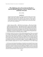
This section reports the results of DD and KS tests. Figures 4.1 to 4.3 show how the
DD statistics changes over the distribution of returns in the grid for the whole sample
period and two sub-periods respectively. The first-, second- and third-order DD
statistics are denoted as T1, T2 and T3 in the figures below.








Figure 4.1: DD Statistics of S&P 500 and NASDAQ 100 for Risk Averters
from January 1998 to December 2003 (Whole Period)
-20
-15
-10
-5
0
5

10
15
20
25
-0.1 -0.1 -0.1 -0.1 -0 -0 -0 -0
0.01 0.02 0.04 0.05 0.06 0.08 0.09 0.11 0.12
0.13 0.15 0.16
Returns
DD Statistics
T1 T2 T3

108









The plots show that T1 are positive for the negative returns and negative for
the positive returns. Most of the T1 are significant for both sides of returns. This
implies that the non-satiation investors prefer old economy stocks when the returns
are negative. On the other hand, when the returns are positive, they would prefer new
economy stocks. This can be attributed to some investors prefer old economy stocks
because of less downside risk. Ang, Chen and Xing (2001) define “downside risk” to
Figure 4.2: DD Statistics of S&P 500 and NASDAQ 100 for Risk Averters
from 1/1/1998 to 09/03/2000 (Bull Sub-period)
-15

-10
-5
0
5
10
15
-0.1 -0.1 -0.1 -0.1 -0.1 -0.1 -0.1 -0 -0 -0 -0 -0 -0
0.01 0.02 0.02
0.03 0.04 0.05 0.06
Returns
DD Statistics
T1 T2 T3
Figure 4.3: DD Statistics of S&P 500 and NASDAQ 100 for Risk Averters
from 10/03/2000 to 31/12/2003 (Bear Sub-period)
-15
-10
-5
0
5
10
15
20
-0.1 -0.1 -0.1 -0.1 -0 -0 -0 -0
0.01 0.02 0.04 0.05 0.07 0.08 0.09 0.11
0.12 0.13 0.15 0.16
Returns
DD Statistics
T1 T2 T3

109

be the risk that an asset’s return is highly correlated with the market when the market
is declining. Markowitz (1959) raises the possibility that agents care about downside
risk, rather than about the market risk. If investors dislike downside risk, then an asset
with greater downside risk is not as desirable as, and should have a higher expected
return than an asset with lower downside risk. On the other hand, all T2 and T3 are
positive and most are significant at 5% significant level for the whole sample period
and bear sub-period. However, it is noted that T2 is negative and significant in the last
15% of the distribution in the bull sub-period. This last 15% of the returns’
distribution is with daily returns of more than 3.8%. Hence, this infers that with very
high returns, the new economy stocks can attract risk-averse investors even they know
it involves high risk to invest in Internet stocks.


Table 4.2: DD Test Results for Risk Averters in Whole Sample Period and
Two Sub-Periods

Sample Period DD FSD SSD TSD
% DD < 0 28 0 0
Whole Period
% DD > 0 26 36 81
% DD < 0 28 17 0
Bull Sub-Period
% DD > 0 23 30 36
% DD < 0 27 0 0
Bear Sub-Period
% DD > 0 27 42 83
Note: % DD < (>) 0 denote the percentage of DD statistics which are significantly negative (positive)
at the 5% significance level, based on the asymptotic critical value of the studentized maximum
modulus (SMM) distribution.

110
Results of the DD test are shown in Table 4.2. Recall that the DD test rejects
the null hypothesis if none of the DD statistics is significantly positive and at least
some (even one) of the DD statistics are significantly negative (DD 2000). However,
this is too restricted as in some situations when
X dominates Y in a small range but
most risk averters will prefer
Y to X (Leshno and Levy 2002). To overcome this
limitation, a 10% cut off point is used in this study. That is, new economy stocks
dominate old economy stocks if at least 10% of the DD statistics are significantly
negative and no DD statistics are significantly positive. Alternatively, if at least 10%
of the DD statistics are significantly positive and no DD statistics are significantly
negative, it is inferred that old economy stocks dominate new economy stocks.

The results show that neither S&P 500 nor NASDAQ 100 dominates each
other at first order for the whole sample period and the two sub periods. Surprisingly,
there is no evidence of NASDAQ 100 dominance even during the Internet boom.
These results are interesting because they indicate that new economy stocks may not
be consistently profitable even in the boom market. There are about half of negative
returns for NASDAQ 100 in the sample period (Table 4.4). On the other hand, the old
economy stocks are more attractive after the crash suggests that (a) investors believe
that old stocks are still better than new stocks and (b) investors have learned from the
earlier period concerning the high risk of Internet stocks.

111

Table 4.3: KS Test Results for Risk Averters in Whole Sample Period and
Two Sub-Periods

Sample Period
Hypotheses FSD SSD TSD
PQ
s
f
0.0000
*
0.0000
*
0.0000
*

Whole Period
QP
s
f

0.0000
*

0.4260 0.6680
PQ
s
f
0.0008
*
0.0000
*
0.0000
*

Bull Sub-Period
QP
s
f
0.0000
*
0.0000
*
0.6610
PQ
s
f
0.0000
*
0.0000
*
0.0000
*

Bear Sub-Period
QP
s
f
0.0000
*
0.6970 0.6600
Note: PQ
s
f means New Economy dominates Old Economy at the s order and vice versa.
*
significant at 1% level,
**
significant at 5% level,
***
significant at 10% level.


Results of the KS test are shown in Table 4.3. The table reports
p-values of the
KS test for first-, second- and third-order SD respectively. Along the row of
PQ
s
f

shows
p-values for testing the hypothesis that new economy stocks weakly dominate
old economy stocks at order
s = 1, 2, 3, while the row QP
s

f tests the opposite
hypothesis. All
p-values are computed by simulations based on the procedure in
Barrett and Donald (2003).

The significance of both hypotheses at first-order SD invalidates the
hypotheses that new economy stocks dominate old economy stocks and vice-versa.
The
p-values for
QP
2
f
and
QP
3
f
are well above 5% (except for second-order
SD in the bull sub-period) while
p-values for the opposite hypotheses are virtually

112
zero across all periods. Thus, there is strong evidence of old economy stocks
dominance over the entire sample period at the second and third orders. These results
strongly indicate that all risk-averse investors would have preferred old economy
stocks over the entire sample period and after the bubble burst. Evidence for old
economy stocks dominance at third-order SD implies that investors who prefer more
positive skewness would also have chosen to buy old economy stocks to maximize
their utility.

Consistent with the DD test results, the KS test shows clear evidence of old

economy stocks dominance. This may imply that there are some rational investors
who prefer old economy stocks than the new economy stocks which are undervalued
by the irrational investors. Although the market has attracted many inexperience
investors or speculators during the extraordinary asset pricing period, the evidence of
old economy stocks dominates even stronger after the bubble burst.

Recall that S&P 500 dominates at the negative returns while NASDAQ 100
dominates at the positive returns. Therefore, it is intended to analyze the descriptive
of negative and positive returns for each index respectively. Table 4.4 displays the
descriptive statistics of daily negative and positive returns for S&P 500 and NASDAQ
100. Both indices have been observed to represent about half of the daily negative and
positive returns respectively for the whole sample period and also during two sub-
periods. S&P 500 has smaller mean (in absolute value) of negative returns and
positive returns respectively than NASDAQ 100 for all periods. The means of
negative and positive returns for NASDAQ 100 are about double the mean returns for
S&P 500. This appears that new economy stocks earn more and lose more than the

113
old economy stocks. Moreover, the probability of getting negative and positive
returns is almost equal in both economies.

Table 4.4: Descriptive Statistics of Daily Negative and Positive Returns for Indices

S&P500- NASDAQ100- S&P500+ NASDAQ100+
Whole Period
mean -0.0100 -0.0214 0.0094 0.0180
t-stat -31.38
*
-32.79
*

30.28
*
29.39
*

median -0.0076 -0.0177 0.0071 0.0132
std. deviation 0.0087 0.0174 0.0088 0.0180
skewness -1.7327 -1.2957 1.7113 2.1949
kurtosis 5.3672 2.3033 3.9261 9.0971
sample size 751 705 813 859
Bull Sub-Period
mean -0.0092 -0.0179 0.0088 0.0156
t-stat -16.86
*
-18.20
*
20.15
*
22.45
*

median -0.0067 -0.0150 0.0071 0.0125
std. deviation 0.0088 0.0146 0.0077 0.0130
skewness -2.2556 -1.6485 1.5452 1.0719
kurtosis 9.3585 5.2658 3.6922 0.9623
Sample size 257 220 313 350
Bear Sub-Period
mean -0.0103 -0.0231 0.0097 0.0197
t-stat -26.59
*

-27.79
*
23.07
*
21.62
*

median -0.0082 -0.0196 0.0072 0.0135
std. deviation 0.0086 0.0183 0.0094 0.0206
skewness -1.4703 -1.1467 1.7113 2.1466
kurtosis 3.4346 1.5802 3.6152 7.8569
Sample size 494 485 500 509
Note: * 1% significant level.
S&P 500- indicates daily negative returns for S&P 500.
NASDAQ 100- indicates daily negative returns for NASDAQ 100.
S&P 500+ indicates daily positive returns for S&P 500.
NASDAQ 100+ indicates daily positive returns for NASDAQ 100.


There are many different approaches that can be applied to study the moment
issue. The DD test is used to study the moment issue as DD test provides additional
information from the whole range of returns distribution for both new and old stocks.
Moreover, the DD test can be used in any correlation situations, and is neither

114
restricted to independent nor pairwise distributions. To investigate the correlation
between new and old stocks, correlation analysis is applied and it has been found that
the correlation between new and old stocks is 0.8342 for the whole period, 0.8308 for
the bull sub-period and 0.8405 for the bear sub-period respectively with 1%
significance level. This finding shows that new and old stocks are highly correlated

but not perfectly correlated and the correlation is consistent for both sub-periods. To
further analyze the micro information about the correlation of the distribution of
returns for both new and old stocks; first, the whole distribution is divided (the whole
range is obtained by combining both new and old stocks) into three equal-distance
intervals for positive returns and three equal-distance intervals for negative returns.
Then, label the intervals to be 1 to 3 from the least positive returns to the most
positive returns and -1 to -3 from the least negative returns to the most negative
returns. The two series of old and new stocks returns are grouped according to the
criteria above for the whole period and two sub-periods. The results are presented in
the 6*6 contingency tables below.


Table 4.5a: Contingency Table for Old Stocks by New Stocks for Whole Period


New Stocks

Rank
-3 -2 -1 1 2 3
Total
-3
1 0 0 0 0 0 1
-2
4 6 1 0 0 0 11
-1
11 116 516 151 1 0 795
1
1 2 103 620 30 1 757
2
0 0 0 0 0 0 0

Old
Stocks
3
0 0 0 0 0 0 0

Total 17 124 620 771 31 1 1564

Chi-Square = 961.57

115





Table 4.5b: Contingency Table for Old Stocks by New Stocks for Bull Sub-Period


New Stocks

Rank
-3 -2 -1 1 2 3
Total
-3
1 0 0 0 0 0 1
-2
0 3 0 0 0 0 3
-1
0 21 180 69 2 0 272
1

0 1 32 162 74 4 273
2
0 0 0 1 11 8 20
Old
Stocks
3
0 0 0 0 0 1 1

Total 1 25 212 232 87 13 570

Chi-Square = 1073





Table 4.5c: Contingency Table for Old Stocks by New Stocks for Bear Sub-Period


New Stocks

Rank
-3 -2 -1 1 2 3
Total
-3
0 0 0 0 0 0 0
-2
4 3 2 0 0 0 9
-1
11 97 333 80 1 0 522

1
1 1 71 362 27 1 463
2
0 0 0 0 0 0 0
Old
Stocks
3
0 0 0 0 0 0 0

Total 16 101 406 442 28 1 994

Chi-Square = 588.25