A study of hitting times for random walks on finite, undirected graphs
Bạn đang xem bản rút gọn của tài liệu. Xem và tải ngay bản đầy đủ của tài liệu tại đây (704.1 KB, 49 trang )
Signature removed
A STUDY OF HITTING TIMES FOR RANDOM WALKS ON
FINITE, UNDIRECTED GRAPHS
by
ARI BINDER
STEVEN J. MILLER, ADVISOR
A thesis submitted in partial fulfillment
of the requirements for the
Degree of Bachelor of Arts with Honors
in Mathematics
WILLIAMS COLLEGE
Williamstown, Massachusetts
April 27, 2011
1
ABSTRACT
This thesis applies algebraic graph theory to random walks. Using the concept of a
graph’s fundamental matrix and the method of spectral decomposition, we derive a formula
that calculates expected hitting times for discrete-time random walks on finite, undirected,
strongly connected graphs. We arrive at this formula independently of existing literature,
and do so in a clearer and more explicit manner than previous works. Additionally we apply
primitive roots of unity to the calculation of expected hitting times for random walks on
circulant graphs. The thesis ends by discussing the difficulty of generalizing these results
to higher moments of hitting time distributions, and using a different approach that makes
use of the Catalan numbers to investigate hitting time probabilities for random walks on
the integer number line.
2
ACKNOWLEDGEMENTS
I would like to thank Professor Steven J. Miller for being a truly exceptional advisor and
mentor. His energetic support and sharp insights have contributed immeasurably both to
this project and to my mathematical education over the past three years. I also thank the
second reader, Professor Mihai Stoiciu, for providing helpful comments on earlier drafts.
I began this project in the summer of 2008 at the NSF Research Experience for Under-
graduates at Canisius College; I thank Professor Terrence Bisson for his supervision and
guidance throughout this program. I would also like to thank Professor Frank Morgan, who
facilitated the continuation of my REU work by directing me to Professor Miller. Addi-
tionally I thank Professor Thomas Garrity for lending me his copy of Hardy’s Divergent
Series. Finally, I would like to thank the Williams Mathematics Department for providing
me with this research opportunity, and my friends and family, whose support and cama-
raderie helped me tremendously throughout this endeavor.
3
CONTENTS
1. Introduction 4
2. A Theoretical Foundation for Random Walks and Hitting Times 6
2.1. Understanding Random Walks on Graphs in the Context of Markov Chains 6
2.2. Interpreting Hitting Times as a Renewal-Reward Process 8
2.3. Two Basic Results 10
3. A Methodology for Calculating Expected Hitting Times 12
3.1. The Fundamental Matrix and its Role in Determining Expected Hitting Times 12
3.2. Making Sense of the Fundamental Matrix 16
3.3. Toward an Explicit Hitting Time Formula 19
3.4. Applying Roots of Unity to Hitting Times 23
4. Sample Calculations 25
5. Using Catalan Numbers to Quantify Hitting Time Probabilities 30
5.1. The Question of Variance: A Closer Look at Cycles 30
5.2. A Brief Introduction to the Catalan Numbers 32
5.3. Application to Hitting Time Probabilities 34
6. Conclusion 39
7. Appendix 40
References 44
4
1. INTRODUCTION
Random walk theory is a widely studied field of mathematics with many applications,
some of which include household consumption [Ha], electrical networks [Pa-1], and con-
gestion models [Ka]. Examining random walks on graphs in discrete time, we quantify
the expected time it takes for these walks to move from one specified vertex of the graph
to another, and attempt to determine the distribution of these so-called hitting times (see
Definitions 1.9 below) for random walks on the integer number line.
We start by recording basic definitions from graph theory that are relevant to our study,
and providing a basic example. The informed reader can skip this subsection, and the
reader seeking a more rigorous introduction to algebraic graph theory should consult [Bi].
Definitions 1.1. A graph G = (V, E) is a vertex set V combined with an edge set E, where
members of E connect members of V . We say G is an n-vertex graph if |V | = n. By
convention we disallow multiple edges connecting the same two vertices and self-loops;
that is, there is at most one element of E connecting i to j when i = j, and no edges
connecting i to j when i = j, where i, j ∈ V . Furthermore, we call G undirected when an
edge connects i to j if an only if an edge connects j to i.
Unless otherwise specified, we assume G is undirected throughout this paper, and thus
define an edge as a two-way path from i to j where i, j ∈ V and i = j.
Definition 1.2. We say that a graph G is strongly connected if for each vertex i, there exists
at least one path from i to any other vertex j of G.
Definition 1.3. When an undirected edge connects i and j, we say that i and j are adjacent,
or that i and j are neighbors. We denote adjacency as i ∼ j.
Definition 1.4. We call an n-vertex graph k-regular if there are exactly k edges leaving
each vertex, where 1 ≤ k < n and n > 1.
Definition 1.5. The n-vertex graph G is vertex-transitive if its group of automorphisms acts
transitively on its vertex set V . This simply means that all vertices look the same locally,
i.e. we cannot uniquely identify any vertex based on the edges and vertices around it.
Definition 1.6. An n-vertex graph G is bipartite if we can divide V into two disjoint sets
U and W such that no edge in E connects two vertices from U or two vertices from W .
Equivalently, all edges connect a vertex in U to a vertex in W.
5
The undirected 6-cycle, two representations of which are given below in Figure 1, pro-
vides an easy way to visualize the above definitions, and is the example we will be using
throughout the thesis.
FIGURE 1. Two representations of the undirected 6-cycle.
From Definitions 1.2 and 1.4, we can immediately see that the undirected 6-cycle is
strongly connected and 2-regular. Furthermore, Definition 1.5 tells us that the undirected
6-cycle is vertex-transitive, because the labeling of the vertices does not matter. Whatever
labeling we choose, each vertex will still be connected to two other vertices by undirected
edges, and thus labeling is the only way we can uniquely identify each vertex. In fact, if we
assume undirectedness, no multiple edges, and no self-loops, then k-regularity is equivalent
to vertex-transitivity. Finally, from Definition 1.6 and from the graph on the right in Figure
1, we can see that the undirected 6-cycle is bipartite, with disjoint vertex sets U = {1, 3, 5}
and W = {2, 0, 4}.
Definition 1.7. A random walk on an n-vertex graph G is the following process:
• Choose a starting vertex i of G.
• Let A ⊂ V = {j : i ∼ j}. Choose an element j of A uniformly at random.
• If not at the walk’s stopping time (see Definition 2.4 below), move to j, and repeat
the second step. Otherwise end at j.
Definition 1.8. Consider a random walk on an n-vertex graph G, where G is isomorphic
to a bipartite graph. We refer to this phenomenon by saying either that the walk or G is
periodic. If G is not isomorphic to a bipartite graph, then the walk and G are aperiodic.
Thus when referring to G, we use “bipartite” and “periodic” interchangeably. This is
a slight abuse of the terminology: processes are periodic, not graphs. However, we are
6
comfortable describing a graph as periodic in this paper because we only discuss graphs in
the context of random walks.
Note that our definition of a random walk is a discrete time definition. All of the results
in this paper apply to discrete time random walks, but are convertible to continuous time,
according to [Al-F1].
Definitions 1.9. The hitting time for a random walk from vertex i to a destination is the
number of steps it takes the walk to reach the destination starting from i. Define the walk’s
destination as the first time it visits vertex j; then we denote the walk’s expected hitting
time as E
i
[T
j
], and the variance of the walk’s hitting time distribution as V ar
i
[T
j
].
Just as with any other expected value, we can intuitively define E
i
[T
j
] as a weighted
average. Thus E
i
[T
j
] =
∞
n=0
n · P (walk first reaches j starting from i in n steps). We
can define V ar
i
[T
j
] in the same probabilistic manner. Because of the infinite number of
possible random walks we must take into account, calculating E
i
[T
j
] and V ar
i
[T
j
] values
from the probabilistic definition appears to be a very difficult task to carry out. In this
thesis we develop a more tractable method for quantifying hitting time distributions. Our
main result is the use of spectral decomposition of the transition matrix (see Definitions
2.2 below) to produce a natural formula for the calculation of expected hitting times on
n-vertex, undirected, strongly connected graphs. The rest of the thesis is organized as
follows: Section 2 constructs a theoretical conceptualization of hitting times for random
walks on graphs, Section 3 uses spectral decomposition to develop a hitting time formula
and applies primitive roots to the construction of spectra of transition matrices, Section 4
applies our methodology in sample calculations, Section 5 attempts to quantify hitting time
distributions on the number line, and Section 6 concludes.
2. A THEORETICAL FOUNDATION FOR RANDOM WALKS AND HITTING TIMES
In the following subsections, we construct a rigorous framework that both supports nat-
ural observations about random walks on graphs and allows us to move toward our goal
of calculating expected hitting times for random walks on finite graphs. The reader is
instructed to see the literature for proofs of any unproved assertions below.
2.1. Understanding Random Walks on Graphs in the Context of Markov Chains. We
appeal to [No] for the following association of random walks on graphs to discrete time
Markov chains. The following definitions and results are summaries of relevant results
7
from [No], Sections [1.1] and [1.4]. See [Sa] as well for a background on finite Markov
chains.
Definitions 2.1. Let I be a countable set. Denote i ∈ I as a state and I as the state-space.
Furthermore, if ρ = {ρ
i
: i ∈ I} is such that 0 ≤ ρ
i
≤ 1 for all i ∈ I, and
i∈I
ρ
i
= 1,
then ρ is a distribution on I.
Consider a random variable X, and let ρ
i
= P (X = i); then X has distribution ρ,
and takes the value i with probability ρ
i
. Let X
n
refer to the state at time n; introducing
time-dependence allows us to use matrices to conceptualize the process of changing states.
Definitions 2.2. We say that a matrix P = {p
ij
: i, j ∈ I} is stochastic if every row
is a distribution, which is to say that each entry is non-negative and each row sums to 1.
Furthermore, P is a transition matrix if P is stochastic such that p
ij
= P (X
n+1
= j|X
n
=
i), where p
ij
is independent of X
0
, . . . , X
n−1
. We express P (X
n
= j|X
0
= i) as p
(n)
ij
.
Definition 2.3. (See Theorem [1.1.1] of [No]). A Markov chain is a set {X
n
} such that
X
0
has distribution ρ, and the distribution of X
n+1
is given by the i
th
row of the transition
matrix P for n ≥ 0, given that X
n
= i.
Definition 2.4. A random variable S, where 0 ≤ S ≤ ∞, is called a stopping time if the
events {S = n}, where n ≥ 0, depend only on X
1
, . . . , X
n
.
These definitions allow us to introduce a property that is necessary for our conception of
hitting times for random walks on graphs.
Theorem 2.5. (Norrris’s strong Markov property; see Theorem [1.4.2] of [No]). Let {X
n
}
be a Markov chain with initial distribution ρ and transition matrix P , and let S be a stopping
time of {X
n
}. Furthermore, let X
S
= i. Then {X
S+n
} is a Markov chain with initial
distribution δ and transition matrix P , where δ
j
= 1 if j = i, and 0 otherwise.
We now apply random walks on graphs to this Markov chain framework.
Proposition 2.6. Consider a random walk starting at vertex i of an n-vertex graph G. Let
S be a stopping time such that X
S
= i. Then the random walk, together with S, exhibits
Norris’s strong Markov property.
8
Proof. First of all, define X
t
as the position of the walk at time t, t ≥ 0. Trivially, we
see that X
0
= i. Let ρ = {ρ
j
: 1 ≤ j ≤ n}, where ρ
j
= 1 if j = i and 0 otherwise.
Then X
0
has distribution ρ. Furthermore, define P as {p
ij
: 1 ≤ i, j ≤ n} where p
ij
is the
number of edges going from vertex i to j divided by the total number of edges leaving i.
From the definition of a random walk given above, we see that p
ij
= P (X
t+1
= j|X
t
= i).
Furthermore, we calculate p
ij
from the structure of the graph; the positions of the walk
have no bearing on the transition probabilities. Thus p
ij
is independent of X
0
, . . . , X
t−1
.
Then {X
t
} is a Markov chain with initial distribution ρ and transition matrix P .
We now consider S. The event set {S = n} refers to the set of occurrences in which
after n steps, the walk is again at vertex i, where n ≥ 0. Clearly these events depend only
on the first n steps of the walk; hence S is a stopping time. Thus according to Theorem
2.5, {X
S+t
} is a Markov chain with initial distribution δ
i
= ρ and transition matrix P . ✷
This result is simply saying that the Markov process “begins afresh” after each stopping
time is reached, and is intuitively clear. In the next subsection, we use this framework to
develop a theoretical conception of hitting times for random walks on graphs.
2.2. Interpreting Hitting Times as a Renewal-Reward Process. In accordance with
[Al-F1], we use renewal-reward theory as a way to think about hitting times for random
walks on graphs. Doing so is a prerequisite for all the results we obtain regarding hitting
times. We appeal to [Co] for the following outline of a renewal-reward process.
Definitions 2.7. Let S
1
, S
2
, S
3
, S
4
, . . . be a sequence of positive i.i.d.r.v.s such that 0 <
E[S
i
] < ∞. Denote J
n
=
n
i=1
S
i
as the n
th
jump time and [J
n−1
, J
n
] as the n
th
renewal
interval. Then the random variable (R
t
)
t≥0
such that R
t
= sup{n : J
n
≤ t} is called a
renewal process. R
t
refers to the number of renewals that have occurred by time t. Now
let W
1
, W
2
, W
3
, W
4
, . . . be a sequence of i.i.d.r.v.s such that −∞ < E[W
i
] < ∞. Then
Y
t
=
R
t
i=1
W
i
is a renewal-reward process.
We can see a natural relation between Definitions 2.7 and Markov chains, which we
prove as the following proposition.
Proposition 2.8. Consider a random walk on an n-vertex graph G starting from vertex i.
Consider a sequence of stopping times S
1
, S
2
, S
3
, . . . such that X
S
n
= i for all n ≥ 1. Let
Y
t
refer to the total number of visits to an arbitrary vertex j that have occurred by the most
recent stopping time. Then Y
t
is a renewal-reward process.
9
Proof. Let S
n
refer to the number of steps the walk takes between the (n − 1)
st
and n
th
stopping times, such that X
S
1
+S
2
+ +S
n−1
= X
S
1
+S
2
+ +S
n
= i. Note that by Proposition
2.6, the random walk on G together with the stopping time S
n
satisfies Theorem 2.5, which
is to say that the portion of the walk between the (n − 1)
st
and n
th
stopping times is
independent of all previous portions of the walk. Furthermore, the starting and ending
positions of each portion of the walk between stopping times are the same, and are governed
by the same transition matrix P , also in accordance with the strong Markov property. Thus
S
1
, S
2
, S
3
, S
4
, . . . is a sequence of i.i.d.r.v.s such that 0 < E[S
i
] < ∞.
Now, let J
n
=
n
i=1
S
i
refer to the number of steps the walk has taken by the time
the n
th
stopping time occurs. Furthermore let R
t
= sup{n : J
n
≤ t} be the number of
stopping times that have been reached by time t. Then according to Definitions 2.7, R
t
is
a renewal process. Now let V
n
be the number of visits to vertex j between the (n − 1)
st
and n
th
stopping times. Once again, because the portion of the walk between the (n −1)
st
and n
th
stopping times is independent of all previous portions of the walk; for all n, the
portion of the walk between the (n − 1)
st
and n
th
stopping times share the same start and
endpoints; and the entire walk is governed by transition matrix P , we conclude that V
1
, V
2
,
V
3
, V
4
, . . . is a sequence of i.i.d.r.v.s such that −∞ < E[V
i
] < ∞. Therefore Y
t
=
R
t
i=1
V
i
is a renewal-reward process, and Y
t
is the number of visits to vertex j by the most recent
stopping time. ✷
We now introduce some key insights that allow us to think about how to calculate ex-
pected hitting times on strongly connected finite graphs. The reader is instructed to see
[No] for proofs.
Theorem 2.9. (The Asymptotic Property of Renewal-Reward Processes). Consider renewal-
reward process Y
t
=
R
t
j=1
W
j
as described in Definitions 2.7. Assume the process begins
in state i. Then lim
t→∞
Y
t
t
=
E
i
[W
1
]
E
i
[S
1
]
.
Definitions 2.10. (Irreducibility of the Transition Matrix). If an n-vertex graph G is
strongly connected, then we say its transition matrix P is irreducible. Irreducibility im-
plies the existence of a unique probability distribution π on the n vertices of G such that
π
j
=
n
i=1
π
i
p
ij
for 1 ≤ j ≤ n. We refer to π as the graph’s stable distribution.
Theorem 2.11. (The Ergodic Theorem; see Theorem 1 of [Al-F1]). Let N
j
(t) be the
number of visits to vertex j during times 1, 2, . . . , t. Then for any initial distribution,
t
−1
N
j
(t) → π
j
as t → ∞, where π = (π
1
, . . . , π
j
, . . . , π
n
) is the stable distribution.
10
With these insights, we arrive at a crucial proposition.
Proposition 2.12. (See Proposition 3 of [Al-F1]). Consider a random walk starting at
vertex i on an n-vertex, strongly connected graph G. Furthermore, let S be a stopping time
such that X
S
= i and 0 < E
i
[S] < ∞. Then E
i
[number of visits to j before time S]
= π
j
E
i
[S] for each vertex j.
Proof. We bring the previous results to bear. Consider a sequence of stopping times
S
1
, S
2
, S
3
, . . ., and assume that these stopping times, together with a stopping time S, are
all governed by the same distribution. Let Y
t
refer to the total number of visits to an arbi-
trary vertex j that have occurred by the most recent stopping time. By Proposition 2.8, Y
t
is a renewal-reward process. Then according to the asymptotic property of renewal-reward
processes, lim
t→∞
Y
t
t
=
E
i
[W
1
]
E
i
[S
1
]
. Since S is distributed identically with S
1
, S
2
, S
3
, . . ., re-
place S
1
with S and W
1
with W in the above expression:
lim
t→∞
Y
t
t
=
E
i
[W ]
E
i
[S]
.
Now by Definitions 2.10, because G is strongly connected, its corresponding transition
matrix P is irreducible. Hence we can use the Ergodic Theorem to express the asymptotic
proportion of time the walk spends visiting vertex j:
lim
t→∞
N
j
(t)
t
= π
j
,
where N
j
(t) is the total number of visits to vertex j by the t
th
step of the walk. Note that
N
j
(t) = Y
t
; rather, Y
t
= N
j
(S
most recent
). However, relative to t, N
j
(t) − Y
t
becomes
arbitrarily small as t → ∞. Hence the two limits are equal, and thus we have
E
i
[W ]
E
i
[S]
= π
j
or E
i
[W ] = π
j
E
i
[S]. Noting that W refers to the number of visits to j before stopping time
S, we arrive at our result. ✷
2.3. Two Basic Results. Proposition 2.12 is very useful because as long as S is a stopping
time such that X
S
= i, we can choose S to be whatever we want. By smart choices of
S and clever manipulation, [Al-F1] uses this proposition to prove many useful properties,
some of them regarding expected hitting times. We prove one of these properties below.
11
Result 2.13. (See Lemma 5 of [Al-F1]). Consider a random walk starting from vertex i on
an n-vertex, strongly connected graph G. Define T
+
i
as the first return time to i. Then
E
i
[T
+
i
] =
1
π
i
.
Proof. Substituting i for j and T
+
i
for S in Proposition 2.12, we get
E
i
[number of visits to i before time T
+
i
] = π
i
E
i
[T
+
i
].
We follow [Al-F1]’s convention, and include time 0 and exclude time t in accounting for
the vertices a t-step walk visits. Note that we visit vertex i exactly once by the first return
time: the visit occurs exactly at time 0, since we exclude time T
+
i
. Substituting 1 in for
E
i
[number of visits to i before time T
+
i
], we arrive at our result. ✷
Applying Result 2.13 to k-regular graphs, we can quantify specific hitting times, as
shown below.
Proposition 2.14. Consider an n-vertex, k-regular, undirected, strongly connected graph
G. Let π represent the stable distribution on G’s vertices. Then π is the uniform distribu-
tion.
Proof. First of all, because G is strongly connected, the transition matrix P is irreducible,
which implies the existence of a stable distribution π. To show π is uniform, note that since
G is k-regular, k edges leave each vertex. Furthermore, because G is undirected, we know
that the number of edges leaving vertex i is equal to the number of edges leading to i for
each vertex i of G. Thus P(X
t+1
= j|X
t
= i) = P (X
t+1
= i|X
t
= j). This implies that
p
ij
= p
ji
for 1 ≤ i, j ≤ n, which means that P is symmetric. Furthermore, if i is connected
to j, then p
ij
= p
ji
= 1/k, and p
ij
= p
ji
= 0 otherwise. Because each vertex is connected
to k vertices, we see that each row of P, and hence each column as well by symmetry,
contains k non-zero terms, each equalling 1/k. Now, let π
i
= 1/n for 1 ≤ i ≤ n. We see
that
π
i
=
1
n
= π
j
for 1 ≤ j ≤ n
= k · π
j
·
1
k
= k · π
j
·
1
k
+ (n − k) · π
j
· 0
=
n
j=1
π
j
p
ji
,
12
which is the irreducibility condition. Thus the stable distribution is uniform, and is unique
by Definition 2.10. ✷
From Proposition 2.14 and Result 2.13, we can immediately see that the expected first
return time for undirected, k-regular, strongly connected graphs is simply equal to n, the
number of vertices on the graph:
E
i
[T
+
i
] = n. (2.14a)
From (2.14a) we can infer another result regarding expected hitting times for random walks
on this class of graphs.
Result 2.15. Assume vertices i and j are adjacent. Consider a random walk starting at
vertex j on an n-vertex k-regular undirected graph G. Then E
j
[T
i
] = n − 1.
Proof. Consider a random walk on G starting at vertex i. After one step, the walk is at j
with probability 1/k for all j such that j ∼ i. Thus we see the following:
E
i
[T
+
i
] = n
= 1 +
1
k
i∼j
E
j
[T
i
]
= 1 +
1
k
· k · E
j
[T
i
]
= 1 + E
j
[T
i
],
yielding E
j
[T
i
] = n − 1 for j ∼ i. ✷
When G is regular, it is possible to construct general formulas for E
i
[T
j
] for the cases
when the shortest path from i to j is of length 2 or 3 (see [Pa-2]). In what follows, we work
toward an explicit formula that does not depend on the regularity of G, and yields expected
hitting time values for random walks on any finite, undirected, strongly connected graph.
We employ spectral decomposition of G’s transition matrix to achieve such a formula.
This application of the spectral decomposition of P to hitting times is well-known; see
[Al, Al-F2, Br, Ta], for instance. However, this literature assumes the background we have
just provided, it often gives results in continuous time, and it does not explicitly state a
formula for determining E
i
[T
j
] values. Thus while the following methodology is by no
means novel, by fully deriving and stating the formula that it permits, and by remaining
in discrete time, we present hitting time results in what we believe to be a clearer, more
straightforward, and more intuitive manner than the existing literature.
13
3. A METHODOLOGY FOR CALCULATING EXPECTED HITTING TIMES
3.1. The Fundamental Matrix and its Role in Determining Expected Hitting Times.
With Proposition 2.12 and a clever choice of S, [Al-F1] defines the fundamental matrix,
from which we can calculate expected hitting times for random walks on any graph with
stable distribution π. We paraphrase their ingenuity in this subsection.
Definition 3.1. Consider a graph G with irreducible transition matrix P and stable distri-
bution π. The graph’s fundamental matrix Z is defined as the matrix such that
Z
ij
=
∞
t=0
(p
(t)
ij
− π
j
).
It is verifiable that the fundamental matrix Z has rows summing to 0, and when π is
uniform, constant diagonal entries (proved as Proposition 7.3 in the appendix). These prop-
erties will come into play later in our discussion, especially in manipulating the following
definition.
Definition 3.2. Consider a random walk on an n-vertex graph G in which for each vertex
j, P (walk starts at j) = π
j
. Then we refer to the expected number of steps it takes the
walk to reach vertex i as E
π
[T
i
].
Theorem 3.3. (The Convergence Theorem; See Theorem 2 of [Al-F1]). Consider a Markov
chain {X
n
}. Then P(X
t
= j) → π
j
as t → ∞ for all states j, provided the chain is
aperiodic.
These definitions set us up to prove our first general result about expected hitting times.
Proposition 3.4. (See Lemma 11 of [Al-F1]). For an n-vertex graph G with fundamental
matrix Z and stable distribution π,
E
π
[T
i
] =
Z
ii
π
i
.
Proof. We get at the notion of Z in the following manner. Consider a random walk on
G starting at vertex i. Let t
0
≥ 1 be some arbitrary stopping time and define S as the time
taken by the following process:
• wait time t
0
,
• and then wait, if necessary, until the walk next visits vertex i.
14
Note that after time t
0
, the graph has probability distribution δ, where P(X
t
0
= j) = δ
j
for
1 ≤ j ≤ n. Hence E[S] = t
0
+ E
δ
[T
i
]. Furthermore, note that the number of visits to i by
time t
0
is geometrically distributed, because we can treat X
n
= i as a Bernoulli Trial for
all n from 1 to t
0
−1. Also, it easy to see that the walk makes no visits to i after time t
0
−1
(remember that we do not include time S in our accounting). Therefore we can express
E
i
[N
i
(t
0
)] as the sum of the i to i transition probabilities:
E[N
i
(S)] =
t
0
−1
n=1
p
(n)
ii
+ 1
=
t
0
−1
n=0
p
(n)
ii
because the walk starts at i.
Invoking Proposition 2.12 and setting j = i, we achieve the following expression:
t
0
−1
n=0
p
(n)
ii
= π
i
(t
0
+ E
δ
[T
i
]).
Rearranging, we get
t
0
−1
n=0
(p
(n)
ii
− π
i
) = π
i
E
δ
[T
i
].
Now let t
0
→ ∞. By definition, the left hand term converges to Z
ii
. Furthermore, by the
convergence theorem, as t
0
becomes large, δ approaches π if G is aperiodic. Therefore the
expression becomes Z
ii
= π
i
E
π
[T
i
], and we arrive at our result.
Now let G be periodic. Then by definition X
t
0
oscillates between disjoint vertex subsets
U and W as t
0
→ ∞. Without loss of generality assume that when n is odd, P (X
n
∈
U) = 0 and when n is even, P (X
n
∈ W ) = 0. Thus i ∈ U, meaning that for odd n,
p
(n)
ii
− π
i
= −π
i
, a constant. Hence the infinite series does not converge. However, if we
scale each partial sum by 1/n, these terms become arbitrarily small as n → ∞. Denoting
the m
th
partial sum of the series as s
m
, we see that lim
t
0
→∞
1
t
0
−1
t
0
−1
m=0
s
m
exists. Thus
the series
t
0
−1
n=0
(p
(n)
ii
−π
i
) is Ces`aro summable (see [Har], for instance), and by definition
of Z, the Ces`aro sum is equal to Z
ii
. Considering the right hand side, note that by the
convergence theorem, for odd n, as n → ∞, the distribution of X
n
converges to a stable
distribution on the elements of W; we call this distribution π
W
. Furthermore, for even n,
as n → ∞, the distribution of X
n
converges to a stable distribution on the elements of U;
call this distribution π
U
. Define δ
n
as the distribution of X
n
on the vertices of G; then the
odd terms of the sequence {δ
n
} approach π
W
and the even terms approach π
U
. Consider
15
ρ
n
=
1
n
n
i=0
δ
n
; then for large n,
ρ
n
≈
1
n
n
2
π
W
+
n
2
π
U
=
1
2
(π
W
+ π
U
),
or equivalently,
lim
n→∞
ρ
n
=
1
2
(π
W
+ π
U
).
Hence the Ces`aro average of this sequence exists.
Now, consider a random walk on G that starts from vertex i, where i ∈ U with proba-
bility 1/2, and i ∈ W with probability 1/2. Then from this starting distribution δ
0
, {δ
n
}
converges to π =
1
2
(π
W
+ π
U
), as indicated above. Using Ces`aro summation as above, we
again see that
t
0
−1
n=0
(p
(n)
ii
− π
i
) → Z
ii
for t
0
→ ∞,
where p
ii
refers to the average of the two i to i transition probabilities. Therefore Z
ii
=
π
i
E
π
[T
i
], completing the proof for the periodic case. ✷
Proposition 3.4 allows us to calculate expected hitting times for a random walk to a
specific vertex when the starting vertex is determined by the stable distribution. We seek to
extend this result so that we can determine expected hitting times for explicit walks from
vertex i to vertex j. We use the following lemma to do so.
Lemma 3.5. (See Lemma 7 of [Al-F1]). Consider a random walk on a graph G with stable
distribution π. Then, for j = i,
E
j
[number of visits to j before time T
i
] = π
j
(E
j
[T
i
] + E
i
[T
j
]).
Proof. Assume the walk starts at j. Define S as “the first return to j after the first visit to
i.” Then we have E
j
[S] = E
j
[T
i
] + E
i
[T
j
]. Because there are no visits to i before T
i
and no
visits to j after T
i
by our accounting convention, substitution into Proposition 2.12 yields
the result. ✷
We are now ready to associate Z with explicit hitting times, and do so below.
Proposition 3.6. (See Lemma 12 of [Al-F1]). For an n-vertex graph G with fundamental
matrix Z and stable distribution π,
E
i
[T
j
] =
Z
jj
− Z
ij
π
j
.
16
Proof. We proceed in the same manner as above. Consider a random walk on G starting
at vertex j. Define S as the time taken by the following process:
• wait until the walk first reaches vertex i,
• then wait a further time t
0
,
• and finally wait, if necessary, until the walk returns to j.
Define δ as the probability distribution such that δ
k
= P
k
(X
t
0
= k). Then E
j
[S] =
E
j
[T
i
] + t
0
+ E
δ
T
j
. Furthermore note that between times T
i
and t
0
, the number of visits to
j is geometrically distributed, so
E
j
[N
j
(t
0
)] = E
j
[number of visits to j before time T
i
] +
t
0
−1
t=0
p
(t)
ij
.
Once again we appeal to Proposition 2.12, and by the same reasoning as above, we achieve
E
j
[number of visits to j before time T
i
] +
t
0
−1
t=0
p
(t)
ij
= π
j
(E
j
[T
i
] + t
0
+ E
δ
T
j
).
Subtracting E
j
[number of visits to j before time T
i
] from both sides and appealing to Lemma
3.5, we obtain
t
0
−1
t=0
p
(t)
ij
= π
j
(−E
i
[T
j
] + t
0
+ E
δ
T
j
).
Rearranging yields
t
0
−1
t=0
(p
(t)
ij
− π
j
) = π
j
(E
δ
T
j
− E
i
[T
j
]).
Once again, we let t
0
→ ∞ and end up with
Z
ij
= π
j
(E
π
[T
j
] − E
i
[T
j
]).
Finally, Proposition 3.4 allows us to write
Z
ij
= Z
jj
− π
j
E
i
[T
j
],
and the proof is complete for the aperiodic case. When G is periodic, we employ the same
argument as above, with the addition that if j ∈ U, p
(n)
ij
= 0 for odd n, and if j ∈ W , then
p
(n)
ij
= 0 for even n. ✷
As Aldous and Fill observe in [Al-F1], because hitting time results are transferable to
continuous time, where the periodicity issue does not arise, it is easier to switch to con-
tinuous time to evaluate random walks that are periodic in the discrete case. However, we
believe that remaining in discrete time is fruitful because it gives us a more tangible sense
of the oscillatory nature of discrete time random walks on bipartite graphs.
17
3.2. Making Sense of the Fundamental Matrix. As we can see from the above section
and ultimately from Proposition 3.6, the fundamental matrix is a powerful tool for our pur-
poses, so long as we can determine it. However, for most graphs it is essentially impossible
to calculate the sum of this infinite series, just as it seems difficult to calculate an expected
hitting time from its probabilistic definition. We therefore seek to equate this definition of
Z with a more useable one. To do so, we make use of the following lemma. While the
results of the next two sections are known, we arrive at them independently of the existing
literature.
Lemma 3.7. Let graph G have irreducible transition matrix P. Define P
∞
as the n by n
matrix such that P
∞
ij
= π
j
for all i. Then PP
∞
= P
∞
= P
∞
P . Furthermore, P
∞
P
∞
=
P
∞
.
Proof. Define J
n
as the n column vector of all ones. Thus we have PP
∞
= P J
n
π. Now,
by stochasticity of P , P J
n
= J
n
, so PP
∞
= J
n
π = P
∞
. Similarly, P
∞
P = J
n
πP . Since
P is irreducible, πP = π. So, P
∞
P = J
n
π = P
∞
. To show P
∞
P
∞
= P
∞
, we write the
following:
(P
∞
P
∞
)
ij
= π
1
π
j
+ π
2
π
j
+ ···+ π
n
π
j
= π
j
(π
1
+ π
2
+ ···+ π
n
)
= π
j
because π is a distribution
= P
∞
ij
.
✷
The commutativity of P with respect to P
∞
is a crucial property, and we use it to express
Z in terms of matrices we can easily calculate.
Proposition 3.8. Consider an n-vertex graph G with irreducible transition matrix P and
fundamental matrix Z. Then
∞
t=0
P
t
− P
∞
= Z = (I − (P −P
∞
))
−1
− P
∞
.
Proof. Consider
∞
t=0
(P
t
− P
∞
) and let t = 0. In this case, P
0
− P
∞
= I − P
∞
=
(P −P
∞
)
0
− P
∞
. For t ≥ 1, we appeal to the binomial theorem, and note that (1 + x)
t
=
t
i=0
t
i
x
i
. Now, let x = −1. Clearly
0 = (1 + (−1))
t
=
t
i=0
t
i
(−1)
i
.
18
This means that for t ≥ 1, if we negate every other term of the expansion of (P − P
∞
)
t
,
the coefficients of the terms will sum to 0. Since P and P
∞
commute, this yields
(P −P
∞
)
t
=
t
0
P
t
−
t
1
P
t−1
P
∞
+
t
2
P
t−2
P
2
∞
− ···±
t
t
P
t
∞
=
t
0
P
t
−
t
1
P
∞
+
t
2
P
∞
− ···±
t
t
P
∞
by Lemma 3.7
= P
t
− P
∞
by the binomial theorem.
We get from the second line to the third line above by knowing that the coefficients of the
terms sum to 0, and the first term, P
t
, has coefficient 1. So we now have
∞
t=0
(P
t
− P
∞
) = (P −P
∞
)
0
− P
∞
+
∞
t=1
(P −P
∞
)
t
=
∞
t=0
(P −P
∞
)
t
− P
∞
.
Consider
∞
t=0
(P − P
∞
)
t
. The first term of this geometric series is I, and the common
factor is (P − P
∞
). From linear algebra, we know that geometric series of powers of
the matrix A converge if and only if A’s eigenvalues are strictly less than 1 in absolute
value. Now because P and P
∞
are real and symmetric, the eigenvalues of (P − P
∞
) are
real; furthermore, because P and P
∞
commute, they are simultaneously diagonalizable,
and hence λ
P
i
− λ
P
∞
i
= λ
(P −P
∞
)
i
, where λ
P
i
P = λ
P
i
v and λ
P
∞
i
P = λ
P
∞
i
v, and v is
the eigenvector that corresponds to both λ
P
i
and λ
P
∞
i
. Note that P
∞
has rank 1 and null
space of dimension n − 1; therefore it has the eigenvalue 1 with multiplicity 1 and 0 with
multiplicity n − 1. Let G be aperiodic; then P has eigenvalue 1 with multiplicity 1, and
all other eigenvalues are strictly less than 1 in absolute value. Because P and P
∞
are
doubly stochastic, the only eigenvector v such that Pv = v and P
∞
= P
∞
v is J
n
. Thus
λ
P
1
= λ
P
∞
1
= 1, and λ
(P −P
∞
)
1
= 1−1 = 0. Furthermore, because λ
P
∞
i
= 0 for 2 ≤ i ≤ n
and |λ
P
∞
i
| < 1 for 2 ≤ i ≤ n, we conclude that the eigenvalues of A = (P − P
∞
) are
strictly less than 1 in absolute value. Therefore, from linear algebra, the series converges
to a sum satisfying
(I − A)(I + A + A
2
+ ···) = I.
Because A has eigenvalues all less than 1 in absolute value, (I −A) has all nonzero eigen-
values, and hence is invertible. Thus the sum of the series is (I −A)
−1
= (I −(P −P
∞
))
−1
,
19
completing the proof for the aperiodic case:
Z =
∞
t=0
(P
t
− P
∞
)
=
∞
t=0
(P −P
∞
)
t
− P
∞
= (I − (P −P
∞
))
−1
− P
∞
.
When G is periodic, -1 is an eigenvalue of P, a result which we prove as Proposition 7.2 in
the appendix. Because P and P
∞
are simultaneously diagonalizable, this eigenvalue of -1
from P is paired with an eigenvalue of 0 from P
∞
, and so P −P
∞
has an eigenvalue of -1.
Thus
∞
t=0
(P − P
∞
)
t
oscillates in the limit, which we would expect based on the proof of
Proposition 3.4 for the periodic case. We appeal to Abel summation (see [Har]) to evaluate
this sum. To do so, let 0 < α < 1. Write
∞
t=0
(P
t
− P
∞
)α
t
=
∞
t=0
(P −P
∞
)
t
α
t
− P
∞
from above
=
∞
t=0
(α(P −P
∞
))
t
− P
∞
.
Because |α| < 1, α(P −P
∞
) has eigenvalues all strictly less than 1 in absolute value. Once
again, because α(P −P
∞
) has no eigenvalues equal to 1, (I −α(P −P
∞
)) has all nonzero
eigenvalues and hence is invertible. Therefore the sum
∞
t=0
(P
t
− P
∞
)α
t
converges to
(I − α(P − P
∞
))
−1
− P
∞
. Making use of this equality and noting that the Abel sum of
∞
t=0
(P − P
∞
)
t
is simply the limit of
∞
t=0
(P
t
− P
∞
)α
t
as α approaches 1 from below,
we find that
∞
t=0
(P −P
∞
)
t
= (I − (P −P
∞
))
−1
.
Note that from the proof of Proposition 3.6, the series
∞
t=0
(p
(t)
ij
− P
∞
ij
) is Ces`aro sum-
mable for each i and j, with Ces`aro sum equal to Z
ij
. Hence
n
t=0
(P
t
− P
∞
) is Ces`aro
summable, with Ces`aro sum equal to Z. Because the Abel sum exists and equals the Ces`aro
sum whenever the latter exists, we see that the Abel sum of
n
t=0
(P
t
−P
∞
) is equal to Z,
and therefore Z = (I − (P −P
∞
))
−1
− P
∞
in the periodic case as well. ✷
20
3.3. Toward an Explicit Hitting Time Formula. Using Proposition 3.8 and Proposition
3.6, we can quantify hitting times on any finite, strongly connected graph. However, the
fundamental matrix is an abstract concept that is hard to visualize. It is hard to tell exactly
where the actual values for the hitting times are coming from. Thus it would be nice if
we could determine hitting times straight from the transition matrix, because we obtain the
transition matrix directly from the graph itself. We work toward quantifying first E
π
[T
j
]
values and then E
i
[T
j
] values using only the transition matrix and its spectrum in this
subsection. Doing so requires associating the spectrum of the fundamental matrix with that
of the transition matrix, which we accomplish with the following lemma.
Lemma 3.9. For an n-vertex graph G with irreducible transition matrix P and fundamental
matrix Z, λ
Z
1
= 0, and for 2 ≤ m ≤ n,
λ
Z
m
= (1 − λ
P
m
)
−1
,
where λ
P
m
refers to the m
th
largest eigenvalue of P .
Proof. From Proposition 3.8, we write Z = (I − (P − P
∞
))
−1
− P
∞
. From linear
algebra, we know that if two matrices commute with each other and are symmetric, then
they are simultaneously diagonalizable. To show Z is symmetric, note that P is symmetric
by undirectedness of G, P
∞
is symmetric by uniformity of π, and I is symmetric by defini-
tion. Because differences of symmetric matrices are symmetric and inverses of symmetric
matrices are symmetric, Z = (I − (P −P
∞
))
−1
− P
∞
is symmetric.
We now must show that P and Z commute. By definition, P commutes with I and with
itself, and by Lemma 3.7, P commutes with P
∞
. Thus we have
P Z = P ((I −(P −P
∞
))
−1
− P
∞
) from Proposition 3.8
= P (I − (P − P
∞
))
−1
− P P
∞
by distributivity of matrix multiplication
= P (I − (P − P
∞
))
−1
− P
∞
P by Lemma 3.7.
= (I − (P −P
∞
))
−1
P −P
∞
P because P commutes with I, P
∞
, and itself
= ((I − (P −P
∞
))
−1
− P
∞
)P by distributivity of matrix multiplication
= ZP.
Thus P commutes with Z, meaning that the two are simultaneously diagonalizable. This
implies that for every eigenvalue λ
Z
m
such that Zv = λ
Z
m
v, Pv = λ
P
m
v, where 1 ≤
m ≤ n and v is an eigenvector in the shared eigenspace. Now we know that λ
P
1
= 1 (see
appendix) with eigenvector J
n
. Hence λ
Z
1
is also associated with J
n
. Because Z has rows
summing to 0 and J
n
has constant entries, λ
Z
1
must be 0.
21
For 2 ≤ m ≤ n, simultaneous diagonalizability of P and Z combined with properties of
eigenvalues allows us to write
λ
Z
m
= λ
((I−(P −P
∞
))
−1
−P
∞
)
m
= λ
(I−(P −P
∞
))
−1
m
− λ
P
∞
m
= (λ
I
m
− (λ
P
m
− λ
P
∞
m
))
−1
− λ
P
∞
m
.
As we observed in the proof of Proposition 3.8, λ
P
∞
k
= 0 for 2 ≤ k ≤ n, so we get rid of
these terms and arrive at our result:
(λ
I
m
− (λ
P
m
− λ
P
∞
m
))
−1
− λ
P
∞
m
=(λ
I
m
− λ
P
m
)
−1
=(1 − λ
P
m
)
−1
, which is defined for 2 ≤ m ≤ n.
✷
With this crucial lemma, which provides a natural formula relating the eigenvalues of
Z to those of P , we are in position to explicitly quantify expected hitting times. Recall
that E
π
[T
j
] refers to the expected number of steps it takes a random walk to reach vertex
j in which the starting vertex is determined by the stationary distribution. Thus it makes
intuitive sense to think of these values as an average of hitting times with an explicit starting
vertex. We prove this a priori intuition below.
Proposition 3.10. For a random walk on an n-vertex graph G with irreducible transition
matrix P and uniform stable distribution π, we have
E
π
[T
j
] =
1
n
n
j=1
E
i
[T
j
] =
n
m=2
(1 − λ
P
m
)
−1
= τ for all j.
Proof. By Proposition 3.4, E
π
[T
j
] =
1
π
j
Z
jj
. Because the rows of Z sum to 0, we can
write
E
π
[T
j
] =
1
π
j
Z
jj
−
n
j=1
Z
ij
.
22
Since the diagonal entries of Z are constant when π is uniform, this becomes
E
π
[T
j
] =
1
n
·
1
π
j
n
j=1
(Z
jj
− Z
ij
)
=
1
n
n
j=1
Z
jj
− Z
ij
π
j
=
1
n
n
j=1
E
i
[T
j
] by Proposition 3.6.
Now, when π is uniform, Proposition 3.4 gives E
π
[T
j
] =
1
π
j
Z
jj
= nZ
jj
. Using m in the
same way as in Lemma 3.9, we write
nZ
jj
= T r(Z) because Z has constant diagonal entries for uniform π
=
n
m=1
λ
Z
m
=
n
m=2
λ
Z
m
=
n
m=2
(1 − λ
P
m
)
−1
by Lemma 3.9.
✷
Thus when π is uniform, the average of the expected hitting times for random walks
on G is simply equal to the sum of the fundamental matrix’s eigenvalues; and because
of the natural relation between Z and P , we can easily express this sum in terms of the
eigenvalues of P . This is a very nice result. Spectral decomposition of Z and P allows
us to determine a similarly nice formula for E
i
[T
j
] values, and one that does not rely on
uniformity of π.
Proposition 3.11. For a random walk on an n-vertex graph G with irreducible transition
matrix P , for any vertices i and j,
E
i
[T
j
] =
1
π
j
n
m=2
(1 − λ
P
m
)
−1
u
jm
(u
jm
− u
im
),
where u
jm
refers to the j
th
entry of the eigenvector of P that corresponds to λ
P
m
.
Proof. Recall that Z is symmetric, and from linear algebra we know that symmetric
matrices can be diagonalized by an orthogonal transformation of their eigenvectors and
eigenvalues. Thus Z = UΛU
T
, where U is an n × n matrix whose columns are the unit