The measurement of time and income poverty in korea
Bạn đang xem bản rút gọn của tài liệu. Xem và tải ngay bản đầy đủ của tài liệu tại đây (1.77 MB, 114 trang )
THE MEASUREMENT OF TIME AND INCOME
POVERTY IN KOREA
The Levy Institute Measure of Time and Income Poverty
Ajit Zacharias, Thomas Masterson, and Kijong Kim
August 2014
Final Report
i
Acknowledgements
This document is the final output of the joint research project between the Levy Economics Institute of
Bard College and the Korea Employment Information Service (KEIS), oyment
The research at the Levy Institute was conducted jointly by two programs:
Distribution of Income and Wealth; and, Gender Equality and the Economy. We are grateful for valuable
comments and other inputs from Tae-hee Kwon at the Korean Employment Information Service. We also
gratefully acknowledge the intellectual support rendered by our colleague and Director of the Gender
Equality program at the Institute, Rania Antonopoulos. The financial support by KEIS is fully
acknowledged. The views in this report are those of the authors and do not necessarily reflect the views of
the Korea Employment Information Service, nor the Ministry of Employment and Labor of South Korea.
ii
Contents
List of Figures iii
List of Tables iv
Preface v
Executive Summary vi
1 INTRODUCTION 1
2 MEASUREMENT FRAMEWORK AND EMPIRICAL METHODOLOGY 5
2.1 A model of Time and Income Poverty 5
2.2 Empirical Methodology and Data 11
2.2.1 Statistical Matching 11
2.2.2 Estimating Time Deficits 12
2.2.3 Adjusted Poverty Thresholds 20
3 INCOME AND TIME POVERTY 23
3.1 Hours of Employment, Time Deficits and Earnings 23
3.2 Household Structure, Time Poverty and Income Poverty 30
3.2.1 The LIMTIP Classification of Households 41
3.2.2 The Impact of Childcare Subsidies and Expenditures on Time and Income Poverty 42
4 LABOR FORCE SIMULATION 46
4.1 Individuals 50
4.2 Households 53
5 CONCLUDING REMARKS: SOME POLICY CONSIDERATIONS 57
5.1 Employment 58
5.2 Wage 59
5.3 Service Provision as a Support for Employment 60
5.3.1 Enhancing the Program for Low-income Households 60
5.4 Direct Income Assistance 61
References 63
APPENDIX A: STATISTICAL MATCHING AND MICROSIMULATION 65
APPENDIX B: IMPUTATION OF OUTSOURCED HOURS OF CHILDCARE 100
iii
List of Figures in the Main Text
Figure 1 Threshold Hours of Household Production (Weekly Hours Per Household) 16
Figure 2 Person's Share in the Total Hours of Household Production (Percent) by Sex, Persons 18 to 70
Years of Age 17
Figure 3 Weekly Hours of Employment by Sex, Persons 18 to 70 Years of Age 20
Figure 4 Incidence of Time Poverty by Weekly Hours of Employment and Sex (Percent) 24
Figure 5 Weekly Hours of Required Household Production, by Weekly Hours of Employment and Sex 25
Figure 6 Time Poverty Rate by Earnings Quintile and Sex (Percent) 27
Figure 7 Composition of Earnings Quintile by Sex (Percent) 27
Figure 8 Weekly Hours of Employment and Required Household Production, by Sex and Earnings
Quintile (Average Values) 28
Figure 9 Median Values of the Ratio of Monetized Value of Time Deficit to Earnings, by Sex and
Earnings Quintile 29
Figure 10 Composition of the Time-poor by Weekly Hours of Employment, Earnings Quintile and Sex
(Percent) 30
Figure 11 Time Poverty Rate of Male Employed Heads and Household Production Requirements by
Type of Household (Persons 18 to 70 Years of Age) 33
Figure 12 Hours of Required Household Production of Women (18 to 70 Years Old) by Type of
Household 34
Figure 13 Time Poverty Rates of Employed Single Female Heads and Wives in Dual-Earner Families (18
to 70 Years, Percent) 35
Figure 14 Ratio of LIMTIP Income Deficit to Official Income Deficit, Employed Households by Type of
Household 40
Figure 15 Type of Childcare Arrangements by Employed Households with Young Children (Percent) 43
Figure 16 Time Poverty Rates of Employed Persons (18 to 70 Years of Age) in Households with Young
Children that Outsource Childcare and Other Households (Percent) 44
Figure 17 Time Deficit of Time-poor Persons with and without Childcare Outsourcing (Average Weekly
Hours) 44
iv
List of Tables in the Main Text
Table 1 Ratio of Irregular Employment and the Share of Women 2
Table 2 Surveys Used in Constructing the Levy Institute Measure of Time and Income Poverty 11
Table 3 Thresholds of Personal Maintenance and Nonsubstitutable Household Activities (Weekly
Hours, Persons Aged 18 to 70 Years) 13
Table 4 Comparison of Membership in the Poverty Band and Predicted Presence in the Poverty Band
in KWPS 2009 15
Table 5 Official Poverty Line, 2008 21
Table 6 Household Structure, Rates of Time Poverty and Composition of Time-poor Households by
Household Type (Percent) 31
Table 7 Poverty of Employed Households by Type of Household: Official vs. LIMTIP 36
Table 8 Poverty of Individuals in Employed Households: Official vs. LIMTIP 36
Table 9 Factors Affecting the Hidden Poverty Rate (LIMTIP Minus Official Poverty Rate) of
Employed Households (Percent), by Household Type 38
Table 10 The Composition of the Income-poor and Average Monthly Income Deficit (in 10,000
and as a Percentage of the Poverty Line) by Type of Household 39
Table 11 LIMTIP Classification of Employed Households and Incidence of Time Poverty Among
Employed Households (Percent) 42
Table 12 LIMTIP Classification of Employed Households with Young Children that Outsource
Childcare (Percent) 45
Table 13 Recipient and Donor Pools for Individuals by Sex 48
Table 14 Recipient and Donor Pools for Childcare Assignment 49
Table 15 Time and Income Poverty Status of Individuals Before and After Simulation 51
Table 16 Rates of Time Poverty Among Individuals Receiving Jobs, Before and After Simulation 52
Table 17 Time Deficits of Time-Poor Individuals Before and After Simulation 52
Table 18 Household Time and Income Poverty Rates, Before and After Simulation 54
Table 19 Average Weekly Hours Caring for Young Children and Outsourced Childcare 55
v
Preface
This report presents findings from the research project
conducted by the Levy Economics Institute in collaboration with the Korea Employment
Information Service. At the Levy Institute, the research was conducted jointly by scholars in the
Distribution of Income and Wealth and Gender Equality and the Economy programs. The central
objective of the project is to develop a measure of time and income poverty for the Republic of
Korea that takes into account household production (unpaid work) requirements. Based on this
new measure, estimates of poverty are presented and compared with those calculated according
to the official income poverty lines.
Policies that are in place in Korea to promote gender equality and economic well-being need to
be reconsidered. The reconsideration should be based on a deeper understanding of the linkages
between the functioning of labor markets, unpaid household production activities, and existing
arrangements of social provisioningincluding social care provisioning. Our hope is that the
research reported here and the questions it raises will contribute to this goal.
We wish to express our gratitude to the Korea Employment Information Service for its financial
and intellectual support without which this undertaking would not have been possible. The
results reported here represent our first step in contributing to the understanding of gender
inequality and constraints faced by low-income households in Korea. We plan to conduct
additional research on Korea alone, as well as in developing comparisons between Korea and
other countries as a part of our work on the Levy Institute Measure of Time and Income Poverty.
vi
Executive Summary
Official poverty lines in Korea and other countries ignore the fact that unpaid household
production activities that contribute to the fulfillment of material needs and wants are essential
for the household to reproduce itself as a unit. This omission has consequences. Taking
household production for granted when we measure poverty yields an unacceptably incomplete
picture, and, therefore the estimates based on this omission provide inadequate guidance to
policymakers.
Standard measurements of poverty assume that all households and individuals have enough time
to adequately attend to the needs of household members, including, for example, caring for
childrentasks absolutely necessary for attaining a minimum standard of living. But this
assumption is false. For numerous reasons, some households may not have sufficient time, and
time deficit and cannot afford to cover it by buying market substitutes (e.g., hiring a care
provider), that household will encounter hardships not reflected in the official poverty measure.
To get a more accurate calculus of poverty, we have developed the Levy Institute Measure of
Time and Income Poverty (LIMTIP), a two-dimensional measure that takes into account both the
necessary income and household production time needed to achieve a minimum living standard.
Our estimates for 2008 show that the LIMTIP poverty rate of employed households (i.e.,
households in which either the head or spouse is employed) was about three times higher than
the official poverty rate (7.5 versus 2.6 percent). The gap between the official and LIMTIP
poverty rates was notably higher for nonemployed male head with employed spouse single
female-headed and dual-earner households. Our estimates of the size of the hidden poor
suggest that ignoring time deficits in household production resulted in a serious undercount of
the working poor. The LIMTIP estimates also expose the fact that the income shortfall of the
poor is greater than implied by the official statistics (43446,000 or 1.8
times greater). Just as with the incidence of poverty, the income shortfall was also greater among
dual-earner and single-headed households. These findings suggest that serious consideration
should be given in the design of income support programs to ensure that they (1) broaden their
coverage to include the hidden poor, and (2) increase the level of support to offset the income
vii
shortfall emanating from time deficits. There was a stark gender disparity in the incidence of
time poverty among the employed, even after controlling for the hours of employment. Time
poverty is minuscule among part-time (defined as working less than 35 hours per week) male
workers while it is sizeable among part-time female workers (2 versus 18 percent). Among full-
time workers, the time poverty rate of women is nearly twice that of men (36 versus 70 percent).
This suggests that the source of the gender difference in time poverty does not lie mainly in the
difference in the hours of employment; it lies in the greater share of the household production
activities that women undertake.
The widespread use of childcare services in Korea allows us to assess the impact of the use of
these services on time and income poverty. When we account for the use of childcare services in
our estimates, we see that the income poverty rate of employed households that outsource
childcare falls from 5.9 percent to 3.1 percent, and that time poverty rates also fall, although
more so for income-nonpoor households than for income-poor households. We also find that
time poverty rates for employed individuals with young children that outsource childcare falls
drastically (from 54 percent to 29 percent). Employed men and women in such households
benefit as the incidence of time poverty fell from 43 to 26 percent and from 78 percent to 37
percent, respectively, for men and women.
Rates of time poverty are also markedly different across the (LIMTIP) income poverty line.
Time poverty among income-poor households is much higher than among income-nonpoor (80
versus 55 percent). Similar patterns can also be observed for employed men (71 versus 50
percent) and employed women (85 versus 74 percent). Since other types of social and economic
disadvantages tend to accompany income poverty, it is quite likely that the negative effects of
time poverty will affect the income-poor disproportionately compared to the income-nonpoor.
We also examined the effectiveness of job creation for poverty reduction via a microsimulation
model. The simulated scenario assigns each nonemployed but employable adult a job that best
fits (in a statistical sense) their characteristics (such as age and educational attainment). Under
the prevailing patterns of pay and hours of employment, we found that a substantial number of
individuals would escape income poverty as a result of nonemployed persons receiving
employment: 6.4 percent of individuals (15 to 70 years of age) are in income poverty after the
viii
simulation, compared to 8.2 percent before simulation. It is noteworthy that the simulated rate is
considerably higher than the actual official income poverty rate of 4.3 percent. A large
proportion of those assigned employment in the simulation enter into the ranks of the time-
deficient working poor or near-poor.
Tackling the problems of gender inequality and challenges in the economic well-being of the
low-income working population requires, in addition to creating more jobs, progress toward
establishing a regime of decent wages, regulating the length of the standard workweek, and
adopting other measures, such as childcare provisioning. The crucial problem of income and
time deficits can only be adequately dealt with in such a coherent and integrated manner.
1
1 INTRODUCTION
Two financial crises and the period of jobless growth that followed them have transformed the
economic and social foundations of modern Korea. Massive firm closures and the adoption of
liberal labor market policies since the 1997 Asian financial crisis have undermined the
employment and living conditions of millions of workers.
The liberalization of the
workers: those who hold fixed-term, part-time employment, or work via an indirect hiring
(Kim and Park 2006). Irregular workers, despite the inclusion
of part-time in the definition of this type of arrangement, on average spend almost the same
amount of time on the job every week as regular workers. For instance, in 2009, the average
daily workload was 8.5 hours among regular workers, while it was 8.2 hours among irregular
workers. However, despite the similar workloads, irregular workers earn around 60 percent of
and job experience and
duration, according to the annual Survey on Working Conditions by Type of Employment.
1
Irregular employment has quickly become dominant, as seen in Table 1: the ratio of irregular to
regular employed workers was 36.7 percent in 2001 and grew to 58.7 percent by 2004, after
which the ratio gradually declined to 47.7 percent in 2013, in part due to the weak labor demand
in recent years (Seong 2013). Nonetheless, the ratio remains much higher than in 2001, when
the data was officially published for the first time.
As earnings from employment constitute the most important source of income for the majority
of households, the deteriorating conditions in the labor market raised the poverty rate among
workers (Lee et al. 2008). Most of the working poor consist of irregular workers, and the fact
that the poverty rate of employed persons rose from 8.8 to 9.7 percent between 2006 and 2010
likely reflects a strong effect of irregular employment on poverty (Kim et al. 2011). Yoon
(2010), Seok (2010), and Lee (2010) found evidence that irregular employment with low wages
1
Source: 2009 Survey on Working Conditions by Type of Employment, Ministry of Employment and Labor, South
Korea.
2
increased the likelihood of being poor and lowered the chances of transitioning out of poverty,
even when the irregular worker was not a primary earner in the household.
This transformation of the Korean economy has necessitated more women to enter the labor
trajectory: it was 47.1 percent in 1997, 53.9 percent in 2009, and continued its growth to 55.6
percent in 2013. D
employment rate from 45.2 to 52.2 percent between 1997 and 2009, and reaching 53.9 percent
in 2013. Despite the growing presence of women in the labor market, these numbers are still
below the Organisation for Economic Co-operation and Development (OECD) averages of 62
percent and 57 percent for participation and employment rates, respectively. This is partly due
as
evidenced by the differences in female labor force participation rates by age group. While
almost 70 percent of women in their late 20s and 65 percent of women in their 40s are
economically active, only 55 percent of women in their 30s are (Economically Active
Population Survey, 2010). Gender inequality in the labor markets has also manifested in
them or more were women in most years
since 2001 (Table 1), while this portion has been less than 38 percent among regular workers.
Gender inequality is also observed in household production: among the employed persons
working 36 hours or more a week, women spent more than 2 hours a day on household
management and caring for other family members while men spent only around 30 minutes a
day in 2009. The inequality is just as striking among those who worked less than 36 hours a
week: 3 hours and 26 minutes for women versus 51 minutes for men.
Table 1 Ratio of Irregular Employment and the Share of Women
2001
2002
2003
2004
2005
2006
2007
2008
2009
2010
2011
2012
2013
Irregular
36.7
37.7
48.3
58.7
57.8
55.2
56.0
51.1
53.7
50.0
52.1
50.0
47.7
Women
52.3
49.5
50.4
49.4
50.1
50.4
49.0
50.4
53.4
53.4
53.4
53.7
53.8
Source: Economically Active Population Survey (labor force survey) from various years.
of irregular employment, has surely increased the incidence, as well as the depth, of time
3
deficits among employed persons: too little time is available for the household activities needed
to maintain the minimum quality of life. Time deficits pose a greater challenge for poor
households, which may not be able to afford to substitute for the insufficient time with goods
and services purchased from the market. As women perform the bulk of household production,
regardless of their paid work hours, the time deficits of employed women are large and their
consequences for the quality of life of employed women are likely to be significant.
However, the official poverty measurement in Korea does not account for time deficits and their
effect, as it is based solely on income. The official poverty threshold is intended to represent the
minimum cost of living and is estimated from the household expenditure survey. It is
periodically updated, as the threshold serves as the baseline for public transfers to poor
households. The official measure does not recognize the need for the time to process and
produce goods and services at home, which otherwise are to be purchased in the market. To the
extent that the long hours of paid work interfere with household production, the well-being of
households and their members is expected to be compromised. The consequent degradation of
the quality of life should therefore be accounted for in the measurement of poverty. To the best
of our knowledge, no systematic attempt to account for the time dimension in poverty
measurement has been made in the case of South Korea.
2
We believe that the recent transformations in the conditions of employment and poverty in
Korea warrant, more than ever, a reconsideration of the official measure of poverty. Policies to
combat poverty and promote equality require a deeper and more detailed understanding of the
linkages between conditions of employment, unpaid household production, and existing
arrangements of social provisioningincluding social care provisioning. This nexus creates
distinct binding constraints for different types of households and individuals, and especially for
men and women. Anti-poverty policies will be much more effective if they take this nexus into
account.
2
Noh and Kim (2010) applied the framework of Vickery (1977) to the 1
st
wave of the Korean Welfare Panel Study
that contains recall data on approximate time spent on household activities. The data, however, suffers from a
severe recall bias. Their study also did not consider the role of household composition in determining the required
time for household production.
4
Our measurement framework is used in an attempt to lay bare the time-income nexus and
provide an empirical picture of the problems that it can produce. Customarily, income poverty
incidence is judged by the ability of individuals and households to gain access to some level of
minimum income based on the premise that such access ensures the fulfilment of basic material
needs. However, this approach neglects to take into account the necessary (unpaid) household
production requirements, without which basic needs cannot be fulfilled. In fact, the two are
interdependent and evaluations of standards of living ought to consider both dimensions.
Households differ in terms of their household production requirements because of demographic
differencesprincipally in terms of size and compositionamong them. Households also differ
in terms of the time their members have available to meet the requirements, and it should not be
assumed that all households can meet these requirements. In order to promote gender equality, it
is imperative to understand how labor force participation and earnings interact with household
production responsibilities, as it is already well-established that women contribute a
disproportionate share of unpaid work time.
The rest of the report has the following structure. In the next section, we discuss our measure of
time and income poverty (Section 2). This section also discusses the data and empirical
methodology. Key findings regarding the patterns of time and income poverty are presented
and discussed in Section 3. We then discuss the findings from our microsimulation of the
scenario in which all employable adults in income-poor households receive employment
(Section 4). The concluding section (Section 5) considers the policy implications of the study.
5
2 MEASUREMENT FRAMEWORK AND EMPIRICAL
METHODOLOGY
The purpose of this section is to describe the model underpinning our measurement of time and
income poverty. We also describe the sources of data and methodology that we employed in
implementing the measure.
2.1 A model of Time and Income Poverty
Our model builds on earlier models that explicitly incorporate time constraints into the concept
and measurement of poverty (Vickery 1977; Harvey and Mukhopadhyay 2007). The key
differences between our approach and the earlier models are that we explicitly take into account
intrahousehold disparities in time allocation and do not rely on the standard neoclassical model
of time allocation. A detailed comparison of the alternative models has been discussed
elsewhere (Zacharias 2011). The empirical methodology followed to implement the model has
been elaborated in the context of three Latin American countries (Zacharias, Antonopoulos and
Masterson 2012).
We undertook a revision of the basic model in order to account for the outsourcing of childcare.
Let the time deficit/surplus faced by the working-age individual in household be denoted as
; minimum required time for personal care and nonsubstitutable household activities as ;
the minimum amount of substitutable household production as ; the fraction of the threshold
hours of household production that falls upon the individual as
; and,
is the time spent on
income generation (wage or own-account employment).
To account for the impact of outsourcing of childcare, we also introduce
to represent the free
(i.e., requiring no monetary outlays by the household) outsourced hours of childcare,
the
purchased hours of childcare and
the share of outsourced hours that goes toward relieving
)
(1)
6
In the equation above,
, the time spent on income generation, is defined so as to also include
the time spent on commuting to work, simply to avoid clutter. The threshold value of personal
care reflects the time requirements for certain basic activities such as sleeping, eating and
drinking, personal hygiene, some minimum rest, etc. We also make allowance for some minimal
requirement of time for certain nonsubstitutable household activities (i.e., activities that are, in
general, hard to outsource). The combined total requirements of personal care and
nonsubstitutable activities is represented by .
3
As we discussed earlier, income poverty thresholds in Korea, as in other countries, do not take
into account the fact that people with poverty-level income may not have enough time to engage
in the household production activities that they need to perform in order subsist with that level
of income. The amount of substitutable household production time that is implicit in the poverty
line ( ) varies among households depending on the number of adults and children in the
household.
Numerous studies based on time use surveys have documented that there are well-entrenched
disparities in the division of household production tasks among the members of the household,
especially between the sexes. Women tend to spend far more time in household production
relative to men. Studies based on time use surveys in Korea have shown that women spent over
3 hours a day on household production while men spent only 37 minutes in 2009, according to a
2009 Korean time n
2007; Lee, Kawaguchi and Hamermesh 2012). The parameter
is meant to capture these
3
Vickery (1977, p.46) defined this as the minimum amount of time that the adult member of the household is
hold and interacting with its members if the household is to function as a
made no allowance for this. Burchardt (2008, p.57) included a minimal amount of parental time for children that
might be double-counting, if we include household management activities in the definition of household
production. However, it can also be argued that most of the nonsubstitutable time consists of the time that the
household members spent with each other and that the poverty-level household production (discussed in the next
paragraph in the text) does n
relatively small amount of time and, therefore, either methodological choice would have no appreciable effect on
the substantive findings.
7
disparities. It is the share of an individual in the total time that their household needs to spend in
household production to survive with the poverty level of income.
Free (unpaid) childcare (
) can be rendered by non-household members (e.g., relatives or
friends). Some time use surveys do collect information on care rendered by the respondent to
non-household children but information on hours spent on (unpaid) care of household children
by non-household members is generally not collected.
4
Free childcare can also be provided by
the government either via direct provisioning or noncash transfers. Hours of care received in this
manner are generally not recorded in time use surveys because of their focus on collecting
information on how respondents spend their time.
In the Korean context, the government
operated a means-tested voucher system to enable families to utilize the services of childcare
centers for their children.
5
Purchased hours of childcare (
) are also generally not available in
time use surveys.
6
Both free and purchased hours of childcare can relieve the time deficits that the individual may
face. Hence, they are entered in our equation for time deficit (equation (1) above) with a plus
sign. However, the extent of such relief can differ among the individuals in the household. For
example, sending the child to a childcare center may relieve the caring responsibility shouldered
by a mother more than a father. The parameter
aims to capture such intrahousehold
differences in the apportionment of outsourced childcare.
The difference between the total hours in a week and the sum of the minimum required time that
the individual has to spend on personal care and household production, net of outsourced hours
4
Kim et.al (2011) are some of a few that have attempted to estimate time use of such childcare arrangements, using
the Korean Longitudinal Survey of Women and Families of 2008. They find that only a small percentage of
households, 6.7 percent, use childcare by non-household members. However, there is no information as to if the
care is provided for free or not. Given the insignificant contribution of the particular type of childcare in aggregate
terms, we do not explicitly take it into account in our conceptual model.
5
In 2008, the childcare subsidies were offered to households with income below 100 percent of average urban
households, with varying degrees of support by income levels. As of the end of September, 575,771 children under
age 5 received the subsidies (source: 2008 Childcare Statistics, Bureau of Childcare Policies, Ministry of Health
and Welfare).
6
There is a strong rationale for collecting information regarding the hours of outsourced hours of care (free and
purchased) in time use surveys because they exert a strong influence on individual and family time allocation. Since
this information cannot be collected via the time diaries of the respondents, it has to be collected via a series of
carefully designed questions.
8
of childcare, is the notional time available to them for income generation and leisure. We have
defined the time deficit/surplus accruing to the individual as the excess or deficiency of hours of
income-generating activity compared to the notional available time. To derive the time deficit at
the household level, we add up the time deficits of the individuals in the household:
(2)
Now, if the household has a time deficit (i.e.,
) then it is reasonable to consider that
deficit as a shortfall in time with respect to
; that is, we assume that the household does not
have enough time to perform the minimum required amount of substitutable household
production.
A crucial point to note in this expression is that we are not allowing the time deficit of an
individual in the household to be compensated by the time surplus of another individual in the
same household. This is a sharp contrast to the usual assumption of unitary households found
in the mainstream literature. The significance of the difference can perhaps be illustrated by
considering the time allocation of the husband and wife in a hypothetical family where both are
employed. Suppose that the wife suffers from a time deficit because she has a full-time job and
also performs the major share of housework; and, suppose that the husband has a time surplus
time time deficit to derive the total time deficit for the household would
be equivalent to assuming that the husband automatically changes his behaviour to relieve the
time deficit faced by the wife. In contrast, we assume that no such automatic substitution takes
place within the household, since we do not observe this substitution in operation in the time use
data that we use.
If the minimal assumptions behind the equations set out above are accepted as reasonable, then
it follows that there is a fundamental problem of inequity that is inherent in the poverty
thresholds if the deficits in the necessary amounts of household production are not taken into
account. Consider two households which are identical in all respects, and which also happen to
have an identical amount of money income. Suppose that one household does not have enough
9
time available to devote to the necessary amount of household production while the other
household has the necessary available time. To treat the two households as equally income-poor
or income-nonpoor would be inequitable towards the household with the time deficit.
The problem of inequity can be resolved by revising the income thresholds. If we assume that
the time deficit in question can be compensated by market substitutes, the natural route is to
assess the replacement cost. Since we do take purchased hours of childcare into account, we also
have to include the expenditures incurred for this purpose in altering the thresholds.
Specifically, the purchased hours of childcare to be included in the adjustment of the income
threshold should be capped at the time deficit that the household would have faced without any
childcare expenditure.
7
If we let
denote the purchased hours of childcare to be taken into account in the modification
of the income threshold and
denote the household time deficit in the absence of purchased
childcare we can express the notion discussed above as:
(3)
where:
(4)
and
(5)
7
In the absence of such a cap, we would raise the income threshold of households that can afford to spend on
childcare beyond the hours required to eliminate the time deficit; potentially, we might end up classifying some
officially nonpoor and time-nonpoor households as falling below the LIMTIP income threshold. This would be
self-contradictory in the sense that the LIMTIP income poverty threshold is meant to add to the ranks of the
income-poor only a subset of households that have incomes above the official poverty line and are time-poor.
10
The income poverty threshold is now the sum of the standard poverty line, monetized value of
time deficit, and cost of purchased hours (capped at the time deficit that would have existed in
the absence of purchased hours):
(6)
In the equation above,
is the adjusted (LIMTIP) income threshold,
the official poverty line,
is the hourly replacement cost of household production and
is the hourly cost of childcare.
We allow the cost of childcare to vary across households because the number of young children
requiring childcare can differ across households; there are other factors, too, that can enter into
play here, e.g., the possibility that while some may pay a subsidized rate, others may pay the
average market rate.
The thresholds for time allocation and modified income threshold together constitute a two-
dimensional measure of time and income poverty. We consider the household to be income-
poor if its income,
, is less than its adjusted threshold, and we term the household as
time-poor if any of its members has a time deficit:
(7)
For the individuals in the household, we deem them to be income-poor if the income of the
household to which they belong is less than the adjusted threshold, and we designate them
as time-poor if they have a time deficit:
(8)
The LIMTIP allows us to identify the hidden income-poorhouseholds with income above
the standard threshold but below the modified thresholdwho would be neglected by official
poverty measures and therefore by poverty alleviation initiatives based on the standard income
thresholds. By combining time and income poverty, the LIMTIP generates a four-way
classification of households and individuals: (a) income-poor and time-poor; (b) income-poor
11
and time-nonpoor; (c) income-nonpoor and time-poor; and (d) income-nonpoor and time-
nonpoor.
2.2 Empirical Methodology and Data
2.2.1 Statistical Matching
The measurement of time and income poverty requires microdata on individuals and households
with information on time spent on household production, time spent on employment, and
household income. Given the importance of intrahousehold division of labor in our model, it is
necessary to have information on the time spent on household production by all persons
8
in
multi-person households. Good data on all the relevant information required are not available in
a single survey. But, good information on household production was available in the time use
survey (KTUS 2009), and good information regarding time spent on employment and household
income was available in the Korean welfare panel survey of 2009.
9
Our strategy was to
statistically match the welfare survey and KTUS surveys so that hours of household production
can be imputed for each individual aged 10 years and older in the welfare survey.
10
Basic
information regarding the surveys is shown in Table 2.
Table 2 Surveys Used in Constructing the Levy Institute Measure of Time and Income Poverty
Survey subject
Name
Sample size
Income and earnings
Korea Welfare Panel Study, 2009
16,255 persons in 6,207 households.
There were 14,502 individuals aged
10 years or older.
Time use
Time Use Survey, Korea, 2009
22,812 persons in 10,639 households.
Completed time diaries were
available for 20,263 individuals that
were 10 years or older.
8
Our basic concern is that we should have information regarding household production by both spouses (partners)
in married-couple (cohabitating) households, and information on older children, relatives (e.g., aunt), and older
adults (e.g., grandmother) in multi-person households.
9
More information on the preparation of the two data files for the purposes of our study is in the report
10
The universe of the KTUS 2009 consisted of persons 10 years and older.
12
The surveys are combined to create the synthetic file using constrained statistical matching
(Kum and Masterson 2010). The basic idea behind the technique is to transfer information from
one survey (donor file) to another (recipient file). In this study, the donor file is the time use
survey and the recipient file is the welfare survey. Time allocation information is missing in the
recipient file but is necessary for our research purposes. Each individual record in the recipient
file is matched with a record in the donor file, where a match represents a similar record, based
on several common variables in both files. The variables are hierarchically organized to create
the matching cells for matching procedure. Some of these variables are considered as strata
variables (i.e., categorical variables that we consider to be of the greatest importance in
designing the match). For example, if we use sex and employment status as strata variables, this
would mean that we would match only individuals of the same sex and employment status.
Within the strata, we use a number of variables of secondary importance as match variables. The
matching progresses by rounds in which strata variables are dropped from matching cell
creation in reverse order of importance.
The matching is performed on the basis of the estimated propensity scores derived from the
strata and match variables. For every recipient in the recipient file, an observation in the donor
file is matched with the same or nearest neighbour based on the rank of their propensity scores.
In this match, a penalty weight is assigned to the propensity score according to the size and
ranking of the coefficients of strata variables not used in a particular matching round. The
quality of match is evaluated by comparing the marginal and joint distributions of the variable
of interest in the donor file and the statistically matched file (see Appendix A for a detailed
description of the statistical matches).
2.2.2 Estimating Time Deficits
We estimated time deficits for individuals aged 18 to 70 years. We restrict our attention to
individuals in this age group because they perform the overwhelming bulk of paid work (98
percent) and account for most of the household production labor performed in the economy (84
percent).
13
To estimate time deficits (see equation (2) above), we require information on:
1. weekly hours of required personal maintenance and nonsubstitutable household
production;
2. weekly hours of required substitutable household production;
3. actual weekly hours of free and purchased childcare;
4. actual weekly hours the individual spends on income generation; and
5. required weekly hours of commuting.
The hours of required personal maintenance were estimated as the sum of minimum necessary
leisure time (assumed to be equal to 14 hours per week)
11
and the weekly average (for all
individuals aged 18 to 70 years) of the time spent on essential activities of personal care,
estimated using data from the time use survey.
12
We assumed that the hours of nonsubstitutable
household activities were equal to 7 hours per week. The resulting estimates are shown below in
Table 3. The line labelled Total is our estimate of the weekly hours of required personal
maintenance and nonsubstitutable household production, and applies uniformly to every adult.
Table 3 Thresholds of Personal Maintenance and Nonsubstitutable Household Activities (Weekly
Hours, Persons Aged 18 to 70 Years)
Personal maintenance
90
Personal care
76
Sleep
54
Eating and drinking
12
Hygiene and dressing
8
Rest
2
Necessary minimum leisure
14
Nonsubstitutable household activities
7
Total
97
Source: KTUS 2009
11
It should be noted that 14 hours per week was approximately 17.5 hours less than the median value of the time
spent on leisure (sum of time spent on social, cultural activities, entertainment, sports, hobbies, games and mass
media). We preferred to set the threshold at a substantially lower level than the observed value for the average
minimum leisure.
12
The KTUS contained two diaries for each respondent. We multiplied the time allocated (measured in minutes) to
each activity in each diary by a conversion factor and then added up the amounts of time spent on the activity over
the two diaries. The conversion factor was set equal to: (a) 3.5 if both diaries were completed on weekdays or
weekends (Saturday and Sunday); and (b) 5 for the weekday diary and 2 for the weekend diary if the two diaries
were completed, respectively, on a weekday and weekend day (Saturday or Sunday). We converted the total weekly
minutes spent on each activity into weekly hours by dividing by 60.
14
The hours of required household production depend on the household-level threshold of
-level threshold. The
thresholds for household production hours are set at the household level; that is, they refer to the
total weekly hours of household production to be performed by the members of the household,
taken together. In principle, they represent the average amount of household production that is
required to subsist at the poverty level of income. The reference group in constructing the
thresholds consists of households with at least one nonemployed adult and income around the
poverty line. Our definition of the reference group is motivated by the need to estimate the
amount of household production implicit in the official poverty line. Since poor households in
which all adults are employed may not be able to spend the amount of household production
implicit in the poverty line, we excluded such households from our definition of the reference
group.
Unfortunately, our preferred source of data for estimating the thresholds, the time use survey,
did not contain any information regarding the income poverty status of households. Therefore,
we had to impute membership in the group of households with income around the poverty line.
We did this by using the predicted probability of being within the poverty band by means of a
probit estimation.
We begin by constructing a household income measure for households in the time use data. For
each individual, we create a personal income variable using the midpoint of the categories of the
household. This results in a household income distribution in the time use data that has a
normalize the household income data in the welfare and time use data separately, in order to
produce similar distributions for the probit estimation and prediction.
We then proceed to run probit estimations on each of the reference group categories for the
required household production (12 combinations of number of adults [one to three or more] and
number of children [zero to three or more] in the household) in the KWPS. The dependent
variable is an indicator of presence in the poverty band and the independent variables are
15
standardized household income, number of persons in the household, a set of dummies for seven
regions of the country, the sex of the household head, the age and square of age of the
household head, dummies for family type, dummies for tenure status, dummies for the type of
housing unit, the number of earners in the household, and the level of education of the
household head. The results of the estimation are used to predict the presence of the household
in the poverty band for all household records in both the time use and the welfare data. We
estimate the latter in order to assess the quality of the procedure. The results for the procedure
are presented in Table 4. As we can see, the rate of misprediction is quite low, at 8.5 percent. In
addition, the highest income of those households in the welfare data that were miscategorized as
t too far above the maximum
imputed membership status of households in the poverty band was used to identify the reference
group in the time use survey.
Table 4 Comparison of Membership in the Poverty Band and Predicted Presence in the Poverty
Band in KWPS 2009
Note: .
We divided the reference group into 12 subgroups based on the number of children (0, 1, 2, and
3 or more) and number of adults (1, 2, and 3 or more) for calculating the thresholds. The
thresholds were calculated on the basis of the average values of the time spent on household
production by households in each subgroup of the reference group. The estimates obtained are
shown below in Figure 1.
Predicted Poverty
0 1
0 80.63 4.05 84.68
1 4.44 10.88 15.32
Total 85.07 14.93 100
Total
Poverty
Band
16
Figure 1 Threshold Hours of Household Production (Weekly Hours Per Household)
Source: KTUS 2009, with the membership in the income-poverty band
Our assumption is that the required hours should show a positive gradient with respect to adults
and a positive gradient with respect to children. That is, the hours of required household
production for the household as a whole should increase when there are more adults in the
household, and when there are more children in the household. We think that this is a reasonable
assumption. Actual hours estimated from the sample data, however, did not satisfy our
assumption in a few cases. This could be due to a variety of reasons.
13
The estimates shown in
Figure 1 were therefore derived on the basis of some adjustments. The first adjustment was
regarding households with one adult and three or more children, which constituted only a small
fraction of all households (about 0.3 percent in 2009). In this case, instead of the estimates
obtained for the reference group, we obtained the threshold by adding to the threshold amount
of the 1-adult+2-kids group, the difference between the threshold amounts of the 2-adult+3-kids
and 2-adults+2 kids subgroups in the reference group. The second adjustment was made for
households with three or more adults and 2 or 3+ children. The number of observations in the
reference group for these subgroups was far too small. To overcome this problem, we relaxed
the criteria for the reference group: enough observations can be found when we drop the
13
Such as small numbers of observations for some of the subgroups in the reference group.
1 adult
2 adults
3+ adults
0
10
20
30
40
50
60
70
80
No child
1 child
2 children
3+
children
Number of children
20
31
47
54
38
51
55
62
51
58
73
78
1 adult
2 adults
3+ adults