A numerical study on iso spiking bifurcations of some neural systems
Bạn đang xem bản rút gọn của tài liệu. Xem và tải ngay bản đầy đủ của tài liệu tại đây (602.52 KB, 62 trang )
A NUMERICAL STUDY ON ISO-SPIKING
BIFURCATIONS OF SOME NEURAL SYSTEMS
CHING MENG HUI
(B.Sc.(Hons.), NUS)
A THESIS SUBMITTED
FOR THE DEGREE OF MASTER OF SCIENCE
DEPARTMENT OF COMPUTATIONAL SCIENCE
NATIONAL UNIVERSITY OF SINGAPORE
2003
Acknow ledgements
This thesis could not have been written without the help of a few people. I am
especially grateful to the following:
Prof. D. B. Creamer, for his guidance and assistance in the culmination of this
thesis.
My supervisors, Prof. Chow Shui-Nee, for his advice and guidance, and Dr. Deng
Bo, for his help and guidance.
My family for their support and encouragement.
My fellow postgraduates, all the staffs and students o f the Department of Compu-
tational Science, Faculty of Science, National University of Singapore.
Oliver Ching
i
Table of Contents
Acknowledgements i
Table of Contents ii
Summary iv
Chapter
1 Introduction 1
1.1 Biological Rhythms And Dynamical Systems . . . . . . . . . . . . . 1
1.2 Preliminaries Of Dynamical Systems And Bifurcation Theo r y . . . . 2
1.3 Preliminaries Of Neural Systems . . . . . . . . . . . . . . . . . . . . 8
2 Iso-Spiking Bif. & Renormalization Uni. 10
2.1 One-Dimensional Return Map . . . . . . . . . . . . . . . . . . . . . 10
2.2 Iso-Spiking Bifurcations . . . . . . . . . . . . . . . . . . . . . . . . 14
2.3 Scaling Laws . . . . . . . . . . . . . . . . . . . . . . . . . . . . . . . 16
2.4 Renormalization Universality . . . . . . . . . . . . . . . . . . . . . 18
3 Numerical Results 25
3.1 Numerical Simulations . . . . . . . . . . . . . . . . . . . . . . . . . 25
3.2 Numerical Results Of Model N . . . . . . . . . . . . . . . . . . . . 26
ii
TABLE OF CONTENTS iii
3.3 Other Models . . . . . . . . . . . . . . . . . . . . . . . . . . . . . . 33
3.3.1 Model A . . . . . . . . . . . . . . . . . . . . . . . . . . . . . 33
3.3.2 Model B . . . . . . . . . . . . . . . . . . . . . . . . . . . . . 34
3.3.3 Model C . . . . . . . . . . . . . . . . . . . . . . . . . . . . . 35
3.3.4 Model D . . . . . . . . . . . . . . . . . . . . . . . . . . . . . 36
3.4 Numerical Results of Model B . . . . . . . . . . . . . . . . . . . . . 37
4 Conclusion 39
Appendix
A Programs v
A.1 Program That Runs The Model-F iles . . . . . . . . . . . . . . . . . v
A.2 Model-File For Model N . . . . . . . . . . . . . . . . . . . . . . . . viii
A.3 Model-File For Model A . . . . . . . . . . . . . . . . . . . . . . . . x
A.4 Model-File For Model B . . . . . . . . . . . . . . . . . . . . . . . . xii
A.5 Model-File For Model C . . . . . . . . . . . . . . . . . . . . . . . . xv
A.6 Model-File For Model D . . . . . . . . . . . . . . . . . . . . . . . . xvii
Bibliography xx
Summary
This thesis is based on a paper by Deng [1], and is written for readers with some
background in Mathematical Analysis. We aim to show, through computer simu-
lations, t he validity of results from [1].
In Chapter One, we touch on the relationship between dynamical systems and
biological science. We also introduce basic co ncepts and definitions in dynamical
systems and neural systems.
In Chapter Two, we review the paper by Deng [1]. We introduce the dynamical
system that was covered in [1]. We look into the iso-spiking bifurcations of the
system and, using some scaling laws and renormalization analysis, we show that
the natural number 1 is a universal constant for any model from the same family
of neural systems.
In Chapter Three, we present the numerical results of the simulation of the system
from Chapter Two. We also detail four other models of systems from [2].
In Chapter Four, we co nclude the thesis with some thoughts of the author.
In the appendix, we provide programs to run simulations of the systems from
Chapters Two and Three. These are all original creations by the author.
iv
Chapter 1
Introduction
In this chapter, we touch on the definitions of terms in dynamical systems.
1.1 Biological Rhythms And Dynamical Systems
In recent years, research has shown that disorderly behaviors in biological rhythms
sometimes appear to follow deterministic rules. This has led to a growing interest
in using nonlinear dynamics in biology, as dynamical systems provide a way of
seeing order and pattern where formerly only the random, the erratic, and the
unpredictable were observed.
As an example, the human body is made up of 10
14
cells, esp ecially neurons, which
are believed to be the key elements in signal processing or communications. The
human brain has 10
11
neurons, and each has more than 10
4
synaptic connections
with other neurons. Neurons by themselves are slow, unreliable analog units, yet
working together, they can carry out highly sophisticated computations in cognition
and control.
By modelling these sophisticated a nd complex biological processes, we can study
the abnormal rhythmic activity in biology systematically. These models can actu-
1
CHAPTER 1. INTRODUCTION 2
ally describ e, to a certain level of accuracy, the actual biological systems. They
exhibit spiking, bursting, chaos, and fractals, by varying parameters of the system.
1.2 Preliminaries Of Dynamical Systems And Bi-
furcation Theory
In this section, we introduce some basic terminology of dynamical systems and
bifurcation theory.
Definition 1.2.1. A dynamical system is a triple {X, t, ϕ}, where X is a state
space, t ∈ R and ϕ
t
: X → X satisfies the properties
ϕ
0
= I,
where I is the identity map on X, that is, I (x) = x for all x ∈ X, and
ϕ
t+s
= ϕ
t
◦ ϕ
s
,
for all t, s ∈ R.
Definition 1.2.2. An orbit starting at x
∗
is a subset of the state space X,
Or (x
∗
) =
x ∈ X : x = ϕ
t
(x
∗
) , t ∈ R
.
Definition 1.2.3. A point x
∗
∈ X is called a n equilibrium (fixed point) if
ϕ
t
(x
∗
) = x
∗
,
for all t ∈ R.
Definition 1.2.4. A point x
∗
∈ X is called a periodic point if
ϕ
t
(x
∗
) = x
∗
,
for some t ∈ R.
CHAPTER 1. INTRODUCTION 3
x
0
0
L
Figure 1.1: Periodic or bit in a
continuous-time system.
L
f
( )
x
0
x
0
f
-1N
( )
x
0
f
2
0
( )
x
0
Figure 1.2: Periodic or bit in a
discrete-time system.
Definition 1.2.5. An orbit, L
0
, is a periodic orbit if each point x
∗
∈ L
0
satisfies
ϕ
t+T
0
(x
∗
) = ϕ
t
(x
∗
) ,
with some T
0
> 0, for all t ∈ R.
Figure 1.1 shows an example of a periodic orbit in a continuous-time system, while
Figure 1.2 presents a periodic o rbit in a discrete-time system.
Definition 1.2.6. A (positively) invariant set of a dynamical system {X, t, ϕ} is
a subset S ⊂ X such that x
∗
∈ S ⇒ ϕ
t
(x
∗
) ∈ S for all t > 0.
Definition 1.2.7. An invariant set S
0
is stable if for any sufficiently small neigh-
borhood U ⊃ S
0
there exists a neighborhood V ⊃ S
0
such that ϕ
t
(x) ∈ U for all
x ∈ V and all t > 0;
Definition 1.2.8. An invariant set S
0
is asymptotically stable if it is stable and
there exists a neighborhood U
0
⊃ S
0
such that ϕ
t
x → S
0
for all x ∈ U
0
, as t → +∞.
Definition 1.2.9. Given a continuous-time dynamical system
˙x = f (x) , x ∈ R
n
, (1.1)
where f is smooth and (1.1) has a periodic orbit L
0
. Take a point x
0
∈ L
0
and
introduce a cross-section Σ to the orbit at this point (see Figure 1.3). An orbit
CHAPTER 1. INTRODUCTION 4
L
x
0
P
x
( )
0
x
Σ
Figure 1.3: The Poincar´e map associated with periodic orbit L
0
.
starting at a point x ∈ Σ sufficiently close to x
0
will return to Σ at some point
˜x ∈ Σ near x
0
. Moreover, nearby orbits will also intersect Σ transversally. Thus, a
map P : Σ → Σ,
x → ˜x = P (x) ,
is constructed. The map P is called a Poincar´e map associated with the periodic
orbit L
0
.
Definition 1.2.10 (Stable Manifold).
W
s
(x
0
) =
x : ϕ
t
x → x
0
, t → +∞
,
is called the stable set of x
0
.
Definition 1.2.11 (Unstable Manifold).
W
u
(x
0
) =
x : ϕ
t
x → x
0
, t → −∞
,
is called the unstable set of x
0
.
Definition 1.2.12. Given a discrete-time dynamical system
x → f (x) , x ∈ R
n
, (1.2)
CHAPTER 1. INTRODUCTION 5
where the map f is smooth along with its inverse f
−1
. Let x
0
= 0 be a fixed
point of the system and let A denote the Jacobian matrix
df
dx
evaluated at x
0
.
The eigenvalues µ
1
, µ
2
, . . . , µ
n
of A are called the multipliers of x
0
. Mulitpliers of
continuous-time dynamical systems are similarly defined.
Definition 1.2.13. A fixed point is called hyperbolic if there are no multipliers on
the unit circle. A hyperbolic equilibrium is called a hyperbolic sad dle if there are
multipliers inside a nd outside the unit circle.
Definition 1.2.14. The appearance of a topologically nonequivalent phase po rtrait
under variation of parameters is called a bifurcation.
Definition 1.2.15. A b i furcation diagram of the dynamical system is a stratifica-
tion of its parameter space induced by t he topological equivalence, together with
representative phase portr aits for each stratum.
Definition 1.2.16. The bifurcation associated with the appearance of a multiplier,
µ
1
= 1 is called a fold (or tangent) bifurcation. This bifurcation is also referred to
as a limit point, saddle-node bifurcation, turning point, among others.
Definition 1.2.17. The bifurcation associated with the appearance of a multiplier,
µ
1
= −1 is called a flip (or period-doubling) bifurcation.
Definition 1.2.18. The bifurcation corresponding to the presence of multipliers,
µ
1. 2
= ±iω
0
, ω
0
> 0, is called a Hopf (or Andronov-Hopf ) bifurcation.
Definition 1.2.19. The bifurcation corresponding to the presence of multipliers,
µ
1, 2
= e
±iθ
0
, 0 < θ
0
< π, is called a Neimark-Sacker (or secondary Hopf ) bifurca-
tion.
Definition 1.2.20. An or bit Γ
0
starting at a point x ∈ R
n
is called homoclinic to
the equilibrium point x
0
of system (1.1) if ϕ
t
x → x
0
as t → ±∞.
CHAPTER 1. INTRODUCTION 6
0
0
x
W
u
W
s
Γ
x
Figure 1.4: Homoclinic orbit on
the plane.
s
x
(2)
Γ
0
(1)
x
x
W
u
W
Figure 1.5: Heteroclinic orbit on
the plane.
Figure 1.6: Homoclinic orbit in three-dimensional space.
Definition 1.2.21. An orbit Γ
0
starting at a point x ∈ R
n
is called heteroclinic to
the equilibrium points x
(1)
and x
(2)
of system (1.1) if ϕ
t
x → x
(1)
as t → −∞ and
ϕ
t
x → x
(2)
as t → +∞.
Figures 1.4 and 1.5 show examples of homoclinic and heteroclinic orbits on the
plane, while Figures 1.6 and 1.7 present relevant examples in the three-dimensional
space. Figure 1.8 shows a homoclinic orbit to a saddle-node equilibrium.
CHAPTER 1. INTRODUCTION 7
Figure 1.7: Heteroclinic orbit in three-dimensional space.
Γ
x
0
x
0
Figure 1.8: Homoclinic orbit Γ
0
to a saddle-node equilibrium.
CHAPTER 1. INTRODUCTION 8
1.3 Preliminaries Of Neural S ystems
In this section, we introduce so me basic terminology associated with neural syst ems.
Definition 1.3.1. Abrupt changes in the electrical potential across a cell’s mem-
brane are ca lled spikes (or action potentials).
Figure 1.9 shows an example of a periodic spiking system.
Definition 1.3.2. A neuron is quiescent if its membrane potential is at r est or
it exhibits small amplitude (“subthreshold”) oscillations. This period of time is
referred to as the silent or quiescent phase.
Definition 1.3.3. When neuron activity alternates between a quiescent state and
repetitive spiking, the neuron activity is said to be bursting.
Figure 1.10 shows an example of a periodic bursting system, depicting the quiescent
and bursting phases.
Definition 1.3.4. Spike number is the number of spikes per burst.
Definition 1.3.5. A neural system is iso-spiking if the spike number is a constant
integer for all bursts.
Figure 1.11 presents an example of an iso-spiking system with spike number 5.
CHAPTER 1. INTRODUCTION 9
0 20 40 60 80 100 120 140 160 180 200
0
0.5
1
1.5
t
V(t)
Figure 1.9: Per iodic spiking sys-
tem.
0 20 40 60 80 100 120 140 160 180 200
−0.5
0
0.5
1
1.5
2
t
V(t)
Bursting
Quiescent State
Quiescent State
Bursting
Figure 1.10: Per iodic bursting
system.
0 50 100 150 200 250 300 350 400
−0.5
0
0.5
1
1.5
2
V(t)
t
Figure 1.11: Iso-spiking system with spike number 5.
Chapter 2
Iso-Spiking Bifurcations and
Renormalization Universality
2.1 One-Dimensio nal Return Map
The following system is the phenomenological model (introduced in [1]) for the
class of neural and excitable cells fo r which the bursting spikes terminates at a
homoclinic o r bit to a saddle point.
Definition 2.1.1. We shall call this system Model N, described as:
dC
dt
= ε (V − ) ,
ς
dn
dt
= (n − n
min
) (n
max
− n) [(V − V
max
) + r
1
(n − n
min
)]
− η
1
(n − r
2
) ,
dV
dt
= (n
max
− n) {(V − V
min
) [V − V
min
− r
3
(C − C
min
)] + η
2
}
− ω (n − n
min
) ,
(2.1)
10
CHAPTER 2. ISO-SPIKING BIF. & RENORMALIZATION UNI. 11
where
r
1
=
V
max
− V
spk
n
max
− n
min
,
r
2
=
n
max
+ n
min
2
,
r
3
=
V
spk
− V
min
C
cpt
− C
min
.
Here n
min
, n
max
, V
min
, V
spk
, V
max
, C
min
, C
cpt
, η
1
, η
2
, ω, ς, ε and are parameters;
in particular, we choo se ε and to be the bifurcation parameters and η
1
, η
2
and ς
are non-negative small parameters which control the multiple time scale processes.
Also
n
min
< n
max
,
V
min
< V
spk
< V
max
,
C
min
< C
cpt
.
In this thesis, we will only consider , such that,
V
min
< < V
spk
,
so that no bursts last forever.
In Model N, (2.1), C is a slow variable for small 0 < ε 1 and corresponds to the
intracellular calcium Ca
2+
concentration. n and V are the fast variables of which
n is fa ster for small 0 < ς 1. n corresponds to the percentage of op en potassium
channels and V corresponds to the cell’s membrane potential.
To apply an extended renormalization theory, we need to reduce the dynamics of
Model N systems to a one-dimensional Poincar´e return map. By the asymptotic
theory of singular perturbations, the dynamics of the perturbed full system with
0 < ς 1 is well approximated by setting ς = 0 (thus defining a flow induced
limiting map). For more details of the derivation of the map and its relation to the
spiking mechanism o f the system, please refer to [1].
CHAPTER 2. ISO-SPIKING BIF. & RENORMALIZATION UNI. 12
−0.2
−0.1
0
0.1
0.2
0.3
0.4
0.5
0
0.2
0.4
0.6
0.8
1
−0.5
0
0.5
1
1.5
2
C(t)
n(t)
V(t)
Figure 2.1: A periodic orbit of Model N with 5 spikes.
Definition 2.1.2. To continue with our quant ita t ive analysis on the spiking dy-
namics, we fit the return map Π as follows:
Π (x) =
ε (
0
−
1
) + x + [1 − ε (
0
−
1
) − c] ×
ε
b
1
||
b
2
1−|x−c|
1+a
1
ε
ε
b
1
||
b
2
+|x−c|
, 0 ≤ x < c,
e
−b
3
/ε
1 −
2x−1
2c−1
1+a
2
ε||
, c ≤ x <
1
2
,
e
−b
3
/ε
1 −
2
|2x − 1|
1+a
2
ε||
,
1
2
≤ x ≤ 1.
(2.2)
where all symbols except fo r are positive parameters subject to the constraints:
V
min
< < V
spk
= 0, 0 <
2
< 1, b
1
> 1, and c =
1
2
+
3
ε.
Note that c is also called the spike termination point.
CHAPTER 2. ISO-SPIKING BIF. & RENORMALIZATION UNI. 13
1
0.5
c
0
1
Figure 2.2: A geometric graph for the return map Π.
As stated and proved by Deng in [1], we list some important properties of (2.2)
that will be needed for the r emaining sections in this chapter.
Property 1.
Π (0) = ε (
0
−
1
) + h.o.t,
where h.o.t denotes terms of higher order than the preceding one. That is,
Π (0) ↓ as ε 0
+
with nonzero asymptotic rate
Π (0) /ε = (
0
−
1
) + h.o.t >
0
,
and
Π (0) ↑ as ↓ .
This is due to the fact that
˙
C = ε (V − ) is the solution through the right continous
limit.
Property 2. The graph of Π over [0, c) must lie above the diagonal line {x
i+1
= x
i
}
as
˙
C = ε (V − ) > 0 for V
min
< < V
spk
≤ V during the active phase of spiking.
Property 3.
lim
ε0
+
Π (x) =
x, 0 ≤ x <
1
2
,
0,
1
2
≤ x ≤ 1,
CHAPTER 2. ISO-SPIKING BIF. & RENORMALIZATION UNI. 14
since every point from [0, C
cpt
) returns to itself at the singular limit ε = 0 and the
asymptotic limit of all the return points of [C
cpt
, 1] goes to 0.
Property 4. The upper bound of Π over [c, 1] decays exponentia lly as ε 0
+
:
max {|Π (x)| : x ∈ [c, 1]} = O
e
−b
3
/ε
.
This exponential scale follows the fact that points of [C
cpt
, 1] is pulled exponentially
to the quiescent branch of the V - nullcline in the variable V and the time required
to pass the turning point in variable C is uniformly bounded from below by an
order of
1
ε
.
2.2 Iso-Spiking Bi fur cations
In this section, we shall derive a criterion for iso-spiking, by following the orbits
through the spike termination point c and the local maximum point C
cpt
.
Definition 2.2.1. Let x
i
min
= Π
i
(c) and x
i
max
= Π
i
(C
cpt
), for i ≥ 1.
Since Π is monotone increasing in [c, C
cpt
], we have
x
1
min
= 0 < x
1
max
.
Assuming
x
2
min
= Π (0) = ε (
0
−
1
) + · · · > x
1
max
= Π (C
cpt
) = O
e
−b
3
/ε
,
is the maximum value of Π in [c, 1]. Note that
Π : [c, 1] →
0, x
1
max
⊂
0, x
2
min
.
Definition 2.2.2. Let N be the fir st largest integer of i such that
x
i
min
< c.
CHAPTER 2. ISO-SPIKING BIF. & RENORMALIZATION UNI. 15
Definition 2.2.3. Let M be t he first largest integer of i such that
x
i
max
< c.
This means that we must have
x
M
min
= 0 < x
M
max
, ⇒ N ≥ M,
since Π is monotone increasing in the spiking interval [0, c).
Now let us consider the two cases.
Case 1 N = M. All the rth iterates, fo r r ≤ N, are in the spiking interval [c, 1),
since x
N
max
< c, and the (N + 1)th iterate is in the quiescent interval [c, 1]
since x
N+1
min
≥ c. Therefore, the spike number for each point of [c, 1] must
be exa ctly N.
Case 2 N > M.
x
1
max
< x
2
min
⇒ x
M+1
max
< x
M+2
min
⇒ N <M + 2
since x
M
max
< c ≤ x
M+1
max
by definition. Therefore, we must have N = M + 1.
Thus implying that there will a difference in the number of iterates in [0, c)
for c and C
cpt
.
So we can now conclude the following criterion.
Iso-Spiking Criterion. The system is iso-spiking if and only if N = M which is
also equivalent to
x
M
max
< c ≤ x
N+1
min
.
Note that the system is non-iso- spiking if and only if N = M + 1.
CHAPTER 2. ISO-SPIKING BIF. & RENORMALIZATION UNI. 16
Definition 2.2.4. Consider the return map (2.2), such that all the parameters
except for ε are fixed, then we have a one-parameter family, which we will denote
by f
ε
.
From this point on till the end o f the chapter, we will consider only ε as our
parameter a nd choose the decreasing direction of ε 0
+
for bifurcation analysis.
Definition 2.2.5. Let α
n
be the first parametric value, such that all paramet-
ric values immediately passing it have spike number n. And let ω
n
be the first
parametric value after α
n
, such that there exists a burst with more than n spikes.
Remark. This means that ω
n
< α
n
and t hat the system must be iso- spiking for
every ω
n
< ε ≤ α
n
.
Definition 2.2.6. The parameter interval (ω
n
, α
n
] is defined as the iso-spiking
interval, I
n
.
Remark. As ε 0
+
, the number of spikes per burst increases and the iterates
x
n
max
, x
n+1
min
decreases. So this means that the parameter value at which x
n
max
first
crosses c from above is the bifurcation point ε = α
n
and x
n+1
min
passes through c
from above is the bifurcation point ε = ω
n
.
This means that we can determine α
n
and ω
n
by the following bifurcation equations:
f
n
α
n
(C
cpt
) = c, f
n
ω
n
(c) = c. (2.3)
2.3 Scaling Law s
To illustrate the quantitative laws that determine the iso-spiking intervals, we
further simplify the return map Π in (2.2).
CHAPTER 2. ISO-SPIKING BIF. & RENORMALIZATION UNI. 17
Definition 2.3.1. Suppose we write
Π (x) = O (ε) + x + L (x)
over the spiking interval [0, c). Induced by the fact that
L (x) = Π (x) − ε (
0
−
1
) − x
⇒ L (x) ∈ O
ε
b
1
−σ
⊂ O (ε)
for b
1
> 2 and outside a radius of some order ε
σ
with 1 < σ < b
1
− 1 from c, we
can drop the term L (x). Denote this simplication by g
ε
, such that
g
ε
(x) = ε + x for x ∈ [0, c) ,
g
ε
(c) = 0,
and
max {g
ε
(x) : x ∈ [c, 1]} = e
−K/ε
for some constant K > 0.
Using (2.3), ω
n
can be calculated explicitly:
g
n+1
ε
(c) = c ⇒ g
n
ε
(0) = c ⇒ nε = c.
Therefore, we have ω
n
=
c
n
for the g
ε
-family, so this leads us to believe that
ω
n
∼
1
n
. (2.4)
Similarly, the (n + 1)th iso-spiking starting point α
n+1
can be calculated:
g
n+1
ε
(C
max
) = c ⇒ g
n
ε
e
−K/ε
= c ⇒ nε + e
−K/
= c,
where C
max
denotes any global maximum point of g
ε
in [c, 1]. Therefore,
α
n+1
=
c
n
−
1
n
e
−Kn/c
+ h.o.t.
CHAPTER 2. ISO-SPIKING BIF. & RENORMALIZATION UNI. 18
So, the length of the nth non-iso-spiking interval is of exponentially small order:
ω
n
− α
n+1
∼
1
n
e
−Kn/c
Thus, in general, we should expect
−1
ln [n (ω
n
− α
n+1
)]
∼
1
n
∼ ω
n
. (2.5)
Therefore we have the interval length ratios:
ω
n+1
− ω
n+2
ω
n
− ω
n+1
,
α
n+2
− ω
n+2
α
n+1
− ω
n+1
∼ 1 −
2
n
. (2.6)
For proofs of (2.4), (2.5) and (2.6), refer to [1].
2.4 Renormalization Universality
In this section, we review [1], where a renormalization argument is presented. The
general idea is to relate
lim
n→∞
ω
n+2
− ω
n+1
ω
n+1
− ω
n
= 1
to an eigenvalue of an operator in a functional space.
We begin with some definitions.
Definition 2.4.1. Let L
1
[0, 1] denote the set of the integrable functions in [0, 1].
Definition 2.4.2. The L
1
norm,
d (g, h) = g − h
1
=
1
0
g (x) − h (x) dx.
Definition 2.4.3. Let F [0, 1] ⊂ L
1
[0, 1], such that,
∀ g ∈ F [0, 1] , ∃ c
0
∈ (0, 1]
such that
g (x) ≥ x for x < c
0
, g (x) ≤ c
0
for x ≥ c
0
,
CHAPTER 2. ISO-SPIKING BIF. & RENORMALIZATION UNI. 19
0
1
1
0
1
R
g
g
c
0
c
−2
c
0
c
−1
1=
c
0
c
0
c
−1
c
0
c
−2
c
0
c
−1
c
0
g
1
c
0
c
0
g
1
c
0
g
c
0
Figure 2.3: A geometric illustration for R.
and either c
0
has a unique preimage c
−1
∈ (0, 1) and satifies
g (x) ≤ c
0
for x < c
−1
, or g (x) ≤ c
0
for x < c
0
.
In the lat t er case, let c
−1
= c
0
for convenience.
Definition 2.4.4. Let an operator R on F [0, 1] be defined by
g ∈ F [0, 1] → R [g] (x) =
1
c
0
g (c
0
x) , 0 ≤ x <
c
−1
c
0
,
1
c
0
g ◦ g (c
0
x) ,
c
−1
c
0
≤ x ≤ 1.
(2.7)
By induction, we can verify the following.
Definition 2.4.5.
R
k
[g] (x) =
1
c
−k+1
g (c
−k+1
x) , 0 ≤ x <
c
−k
c
−k+1
,
1
c
−k+1
g
k+1
(c
−k+1
x) ,
c
−k
c
−k+1
≤ x ≤ 1.
where c
−i
= g
−i
(c
0
) ∈ [0, c
0
) for a ll i = 0, 1, . . . , k. And we will call R
k
[g] the
progression operator.
CHAPTER 2. ISO-SPIKING BIF. & RENORMALIZATION UNI. 20
The following are properties of R, as stated and proved by Deng in [1].
Property 1. If c
0
has n backward iterates,
c
−i
= g
−i
(c
0
) ∈ [0, c
0
) for i = 1, . . . , n,
then the new point
c
−1
c
0
has (n − 1) backward iterates,
c
−j−1
c
0
= R [g]
−j
c
−1
c
0
in
0,
c
−1
c
0
for j = 1, . . . , n − 1.
Property 2. Let
ψ
0
(x) =
x, 0 ≤ x < 1,
0, x = 1.
Then ψ
0
(x) is a fixed point in R, that is,
R [ψ
0
] = ψ
0
.
In fact, for any
ψ
m
(x) =
mx + (1 − m) , 0 ≤ x < 1,
0, x = 1,
for some 0 < m < 1,
R [ψ
m
] = ψ
m
.
Implying that ψ
0
is not isolated and there are other fixed points.
Property 3. Let
ψ
µ
(x) =
µ + x, 0 ≤ x < 1 − µ,
0, 1 − µ ≤ x ≤ 1.
Then we have the following:
(i)
R [ψ
µ
] = ψ
µ/(1−µ)
⇔ R
−1
[ψ
µ
] = ψ
µ/(1+µ)
.