A parent mass filter algorithm for peptide sequencing from tandem mass spectra
Bạn đang xem bản rút gọn của tài liệu. Xem và tải ngay bản đầy đủ của tài liệu tại đây (1.57 MB, 99 trang )
Masters Thesis
A Parent Mass Filter Algorithm for Peptide Sequencing from
Tandem Mass Spectra
By
Tan Huiyi, Max
Department of Computer Science
School of Computing
National University of Singapore
2009/10
Masters Thesis
A Parent Mass Filter Algorithm for Peptide Sequencing from
Tandem Mass Spectra
By
Tan Huiyi, Max
Department of Computer Science
School of Computing
National University of Singapore
2009/10
Project No: HT060752E
Advisor: A/P Leong Hon Wai
Deliverables:
Report: 1 Volume
Abstract
The peptide sequencing problem is that of determining the amino acid sequence of a peptide
from the mass spectrum produced by the peptide via a tandem mass spectrometry process.
This problems has been extensively research in the past decade – the methods are classified as
database search methods or de novo methods.
This thesis focuses on database search methods for peptide sequencing and in particular,
on spectra from the GPM database. Past research [1, 2] have shown that GPM spectra are
particularly challenging as the are many missing peaks and relatively few short sequences, also
known as tags that can be found from these spectra.
This thesis proposes a database search peptide sequencing algorithm, called PMF-MI (Parent
Mass Filter with Mass Index), that work well on sp e ctra with missing peasks and few tags, such
as the GPM database. The main idea in PMF-MI is to use the parent mass as an effective filter
for the set of putative peptides to be considered. Then, this set of putative peptides can be
globally matches against the given spectrum for scoring. This method eliminates the need for
having tags to filter the peptide database.
Similar ideas have been proposed in the past [3]. However, in our work, we push this idea
further by performing a full pre-indexing of all the pe ptides in the database by their parent
masses. This pre-indexing of the peptide database has to be performed only once and based
on current database sizes, the entire index uses only 20GB. A typical parent mass of a given
spectrum will produce a set of about 200,000 putative peptides on average.
We ran our PMF-MI algorithm on the GPM spectra where the annotated peptide agrees
with the precursor peptide mass of the spectra. On this dataset of 877 spectra, our PMF-MI
algorithm is competitive with INSPECT, the state of the art database search method today.
Our PMF-MI recovered 367 correct peptides compared to 376 for INSPECT (based on top 10
ranked results).
One limitation of the PMF-MI is that it requires an accurate parent mass for it to be effective.
To test this hypothesis, we also ran the PMF-MI algorithm on the entire GPM database using
the actual peptide mass of each input spectra
1
. In this case, PMF-MI performed better (577
for PMF-MI compared to 562 for INSPECT).
This observation leads us to the next contribution of the thesis, which is an algorithm to
compute the correct putative parent mass of a given spectrum.
To do this, we examine the peaks which make up the spectra and propose that there are
more pairs of peaks which sum up to the parent mass (with one of the pair representing part of
the protein and the other representing the remaining part) than pairs of peaks which sum up to
any random mass. We supplement our PMF-MI algorithm with this corrected mass and show
that we can now recover 404 correct peptides then compared to 367 correct peptides without
using this corrected mass.
1
To compute the actual peptide mass, we take the sum of the masses of the amino acid which constitutes
the actual peptide that produces the spectra. Note that we are naturally without the benefit of this information
when sequencing an unknown peptide.
Subject Descriptors:
J.3 Life and medical sciences
Keywords:
Bioinformatics, Database Searching, De novo Sequencing, Protein, Peptide, Spectrum, Vi-
sualizer, Peptide, Database, Sequencing, Tags
Implementation Software and Hardware:
• Hardware : PC
• Software : Perl, C#, ASP.NET
iii
Acknowledgement
I would like to thank the Resource Allocation and Scheduling (RAS) Group for all their help
over the past year. Especially the following (not in any order of contribution) -
Associate Professor Leong Hon Wai - for all of his invaluable advice and guidance throughout
the project, the improved tag algorithm would not be possible without him. It was truly a
pleasure working with him.
Chong Ket Fat - for his guidance in the earlier stages of the project, it was tough picking
up all the basics of protein sequencing from scratch and with his help it was a much smo other
and faster progress.
Ning Kang - for explaining to me how his MCPS tag generation algorithm work as well as
his experimental results for comparison purposes.
List of Figures
1.1 Reading a MS/MS output . . . . . . . . . . . . . . . . . . . . . . . . . . . . . . . 4
2.1 Amino Acid Structure . . . . . . . . . . . . . . . . . . . . . . . . . . . . . . . . . 11
2.2 Polypeptide Backbone . . . . . . . . . . . . . . . . . . . . . . . . . . . . . . . . . 12
2.3 Tandem Mass Spectrometer . . . . . . . . . . . . . . . . . . . . . . . . . . . . . . 13
2.4 Sample MS/MS Spectra . . . . . . . . . . . . . . . . . . . . . . . . . . . . . . . . 14
2.5 Fragmentation Points . . . . . . . . . . . . . . . . . . . . . . . . . . . . . . . . . 15
2.6 Formation of the different ion types . . . . . . . . . . . . . . . . . . . . . . . . . . 16
2.7 Internal Ion . . . . . . . . . . . . . . . . . . . . . . . . . . . . . . . . . . . . . . . 16
2.8 Generation of theoretical spectra . . . . . . . . . . . . . . . . . . . . . . . . . . . 22
2.9 Overlaps For Sample Theoretical and Experimental Spectrum . . . . . . . . . . . 25
3.1 DB Search Model . . . . . . . . . . . . . . . . . . . . . . . . . . . . . . . . . . . . 31
3.2 Consecutive Peaks . . . . . . . . . . . . . . . . . . . . . . . . . . . . . . . . . . . 35
3.3 Combined Coverage Sample . . . . . . . . . . . . . . . . . . . . . . . . . . . . . . 37
3.4 Low Probability Peaks . . . . . . . . . . . . . . . . . . . . . . . . . . . . . . . . . 46
3.5 Simple Look-ahead . . . . . . . . . . . . . . . . . . . . . . . . . . . . . . . . . . . 46
4.1 GPM Vs ISB . . . . . . . . . . . . . . . . . . . . . . . . . . . . . . . . . . . . . . 51
4.2 Sample GPM dataset . . . . . . . . . . . . . . . . . . . . . . . . . . . . . . . . . . 52
4.3 DB Search Model (Modified) . . . . . . . . . . . . . . . . . . . . . . . . . . . . . 53
4.4 Building a Tr ie to Reduce Running Time . . . . . . . . . . . . . . . . . . . . . . 56
4.5 Indexing Fragmention Points . . . . . . . . . . . . . . . . . . . . . . . . . . . . . 57
4.6 Comparing Inspect and PMF-MI on filtered GPM datasets . . . . . . . . . . . . 61
4.7 Comparing Inspect and PMF-MI on Full GPM datasets . . . . . . . . . . . . . . 62
4.8 Overlaps For Sample Theoretical and Experimental Spectrum . . . . . . . . . . . 66
5.1 Distribution of GPM and ISB datasets . . . . . . . . . . . . . . . . . . . . . . . . 67
5.2 Cumulative mass difference . . . . . . . . . . . . . . . . . . . . . . . . . . . . . . 70
5.3 Distribution of GPM datasets . . . . . . . . . . . . . . . . . . . . . . . . . . . . . 70
5.4 Distribution of GPM datasets . . . . . . . . . . . . . . . . . . . . . . . . . . . . . 72
5.5 Distribution of GPM datasets . . . . . . . . . . . . . . . . . . . . . . . . . . . . . 73
A.1 The canvas and the tabbed regions. . . . . . . . . . . . . . . . . . . . . . . . . . . A-2
A.2 Default View . . . . . . . . . . . . . . . . . . . . . . . . . . . . . . . . . . . . . . A-3
A.3 Annotation View . . . . . . . . . . . . . . . . . . . . . . . . . . . . . . . . . . . . A-4
A.4 Backtrack View . . . . . . . . . . . . . . . . . . . . . . . . . . . . . . . . . . . . . A-5
A.5 Tag View . . . . . . . . . . . . . . . . . . . . . . . . . . . . . . . . . . . . . . . . A-6
A.6 Pepnovo View . . . . . . . . . . . . . . . . . . . . . . . . . . . . . . . . . . . . . . A-7
A.7 Graph Vis View . . . . . . . . . . . . . . . . . . . . . . . . . . . . . . . . . . . . . A-8
v
List of Tables
2.1 Annotation Set For Pseudo Peaks . . . . . . . . . . . . . . . . . . . . . . . . . . . 20
2.2 Prefix Fragment Overlaps For Various Charges . . . . . . . . . . . . . . . . . . . 26
3.1 Number of true peaks by ion type . . . . . . . . . . . . . . . . . . . . . . . . . . 34
3.2 Number of true peaks by ion type after merging. . . . . . . . . . . . . . . . . . . 35
3.3 Number of consecutive peaks . . . . . . . . . . . . . . . . . . . . . . . . . . . . . 36
3.4 Tag Coverage . . . . . . . . . . . . . . . . . . . . . . . . . . . . . . . . . . . . . . 38
3.5 Table showing the top R results of PepNovo and our algorithm SimTag . . . . . 44
3.6 Table showing the average rank of the correct tags for PepNovo and our algorithm
SimTag . . . . . . . . . . . . . . . . . . . . . . . . . . . . . . . . . . . . . . . . . 44
3.7 Simple lookahead . . . . . . . . . . . . . . . . . . . . . . . . . . . . . . . . . . . . 48
3.8 Simple Lookahead Using Annotation Probability . . . . . . . . . . . . . . . . . . 48
3.9 Summary of Algorithms mentioned . . . . . . . . . . . . . . . . . . . . . . . . . . 49
4.1 Running time after optimization . . . . . . . . . . . . . . . . . . . . . . . . . . . 58
4.2 Using mass fragmentation index as a coarse filter . . . . . . . . . . . . . . . . . . 59
4.3 Sequencing results from Inspect and PMF . . . . . . . . . . . . . . . . . . . . . . 63
4.4 Summary of improvements . . . . . . . . . . . . . . . . . . . . . . . . . . . . . . . 64
5.1 Using real fragment mass . . . . . . . . . . . . . . . . . . . . . . . . . . . . . . . 68
5.2 Explained Post Translational Modifications for Figure 5.3 . . . . . . . . . . . . . 71
5.3 Increase in upper-bound of database search with mass convolution . . . . . . . . 75
5.4 Distribution of GPM datasets . . . . . . . . . . . . . . . . . . . . . . . . . . . . . 76
5.5 Experiments on Full and Convoluted sets. . . . . . . . . . . . . . . . . . . . . . . 77
vi
Table of Contents
Title i
Abstract ii
Acknowledgement iv
List of Figures v
List of Tables vi
1 Introduction 1
1.1 The peptide sequencing problem . . . . . . . . . . . . . . . . . . . . . . . . . . . 2
1.2 Existing work . . . . . . . . . . . . . . . . . . . . . . . . . . . . . . . . . . . . . . 5
1.3 Key contributions in this thesis . . . . . . . . . . . . . . . . . . . . . . . . . . . . 6
1.4 Report organization . . . . . . . . . . . . . . . . . . . . . . . . . . . . . . . . . . 7
2 Overview of research 10
2.1 Background . . . . . . . . . . . . . . . . . . . . . . . . . . . . . . . . . . . . . . . 10
2.2 Mass spectrometer . . . . . . . . . . . . . . . . . . . . . . . . . . . . . . . . . . . 11
2.2.1 Mass spectrum output . . . . . . . . . . . . . . . . . . . . . . . . . . . . . 13
2.2.2 Interpreting the mass spectrum . . . . . . . . . . . . . . . . . . . . . . . . 17
2.3 Modeling the peptide se quencing problem . . . . . . . . . . . . . . . . . . . . . . 18
2.3.1 Theoretical spectrum . . . . . . . . . . . . . . . . . . . . . . . . . . . . . . 19
2.3.2 Extended spectrum . . . . . . . . . . . . . . . . . . . . . . . . . . . . . . . 21
2.4 Extended spectrum graph . . . . . . . . . . . . . . . . . . . . . . . . . . . . . . . 23
2.5 Literature Review . . . . . . . . . . . . . . . . . . . . . . . . . . . . . . . . . . . 24
2.5.1 De novo sequencing methods . . . . . . . . . . . . . . . . . . . . . . . . . 24
2.5.2 Database search methods . . . . . . . . . . . . . . . . . . . . . . . . . . . 28
3 Preliminary research 31
3.1 Data analysis . . . . . . . . . . . . . . . . . . . . . . . . . . . . . . . . . . . . . . 32
3.1.1 Data sets . . . . . . . . . . . . . . . . . . . . . . . . . . . . . . . . . . . . 32
3.1.2 Types of analysis . . . . . . . . . . . . . . . . . . . . . . . . . . . . . . . . 33
3.2 A simple tag generation algorithm . . . . . . . . . . . . . . . . . . . . . . . . . . 39
3.2.1 The Extended Spectrum Graph . . . . . . . . . . . . . . . . . . . . . . . . 39
3.2.2 Tag generation . . . . . . . . . . . . . . . . . . . . . . . . . . . . . . . . . 41
3.2.3 Scanning for matches in the database . . . . . . . . . . . . . . . . . . . . 42
3.2.4 Scoring . . . . . . . . . . . . . . . . . . . . . . . . . . . . . . . . . . . . . 42
3.3 Comparing the different algorithms . . . . . . . . . . . . . . . . . . . . . . . . . . 43
3.3.1 Number of tags found in top R ranks . . . . . . . . . . . . . . . . . . . . 43
vii
3.3.2 Average rank of the first correct tag . . . . . . . . . . . . . . . . . . . . . 43
3.3.3 Preliminary results . . . . . . . . . . . . . . . . . . . . . . . . . . . . . . . 44
3.4 Some enhancements . . . . . . . . . . . . . . . . . . . . . . . . . . . . . . . . . . 45
3.4.1 Using a lookahead strategy for scoring . . . . . . . . . . . . . . . . . . . . 45
3.4.2 Simple look ahead analysis . . . . . . . . . . . . . . . . . . . . . . . . . . 46
3.4.3 Using annotation probability . . . . . . . . . . . . . . . . . . . . . . . . . 47
3.4.4 Conclusion of looking ahead methods in scoring tags . . . . . . . . . . . . 49
4 Database search by parent mass filter 50
4.1 Motivation . . . . . . . . . . . . . . . . . . . . . . . . . . . . . . . . . . . . . . . 50
4.2 Filtering by parent mass . . . . . . . . . . . . . . . . . . . . . . . . . . . . . . . . 51
4.2.1 Optimization 1: building the index by mass . . . . . . . . . . . . . . . . . 53
4.2.2 General method for evaluating candidate sequences . . . . . . . . . . . . . 54
4.3 A scoring function for candidate peptides in PMF-Opt1 . . . . . . . . . . . . . . 55
4.4 Making further improvements in PMF-Opt1 . . . . . . . . . . . . . . . . . . . . . 56
4.4.1 Initial method of using a Trie . . . . . . . . . . . . . . . . . . . . . . . . . 56
4.4.2 Building a mass fragmentation index . . . . . . . . . . . . . . . . . . . . . 57
4.5 Implementation and Datasets . . . . . . . . . . . . . . . . . . . . . . . . . . . . . 59
4.5.1 Conclusion . . . . . . . . . . . . . . . . . . . . . . . . . . . . . . . . . . . 64
5 Parent mass correction by convolution 67
5.1 Introduction . . . . . . . . . . . . . . . . . . . . . . . . . . . . . . . . . . . . . . . 67
5.2 Background . . . . . . . . . . . . . . . . . . . . . . . . . . . . . . . . . . . . . . . 69
5.3 Data analysis for parent mass correction . . . . . . . . . . . . . . . . . . . . . . . 69
5.4 Mass correction by histogram . . . . . . . . . . . . . . . . . . . . . . . . . . . . . 71
5.5 Using the convoluted mass in database search . . . . . . . . . . . . . . . . . . . . 74
5.6 Using the convoluted mass as a measure for spectra quality . . . . . . . . . . . . 75
6 Conclusion 79
References 81
A Spectrum Visualize r A-1
A.1 Implementation and Program Information . . . . . . . . . . . . . . . . . . . . . . A-1
A.1.1 Implementation . . . . . . . . . . . . . . . . . . . . . . . . . . . . . . . . . A-1
A.2 Using the program . . . . . . . . . . . . . . . . . . . . . . . . . . . . . . . . . . . A-2
A.2.1 Program regions . . . . . . . . . . . . . . . . . . . . . . . . . . . . . . . . A-2
A.2.2 Starting the program . . . . . . . . . . . . . . . . . . . . . . . . . . . . . . A-3
A.2.3 Annotation View . . . . . . . . . . . . . . . . . . . . . . . . . . . . . . . . A-4
A.2.4 Backtrack View . . . . . . . . . . . . . . . . . . . . . . . . . . . . . . . . . A-5
A.2.5 Tag View . . . . . . . . . . . . . . . . . . . . . . . . . . . . . . . . . . . . A-6
A.2.6 Pepnovo and GBST View . . . . . . . . . . . . . . . . . . . . . . . . . . . A-7
A.2.7 GraphVis and Simple Graph . . . . . . . . . . . . . . . . . . . . . . . . . A-8
viii
Chapter 1
Introduction
The Human Genome Project was an international scientific research project with the aim of
determining the sequence of nucleotides which makes up DNA and to map the 25000 ge nes of
the human genome. The project began in 1990 and was completed in 2003.
The key benefits of this project was to provide new directions for advances in medicine and
biotechnology. For example, genetic tests is possible to determine the likelihood for cancer,
cystic fibrosis and other diseases. Investigations of hereditary diseases can narrow down the
cause to a target gene. However, since the complete DNA is found in every single cell of our
body (save a few exceptions), the search for the erroneous gene within the 3 billion or so base
pairs of nucleotides effectively becomes a search of a needle in a haystack. The existence of
introns or non coding regions further implicates the problem.
To determine the location of the erroneous DNA, we can investigate the proteins found in
the faulty part of the body. Specific proteins are only expressed in specific parts of the body (For
example, only our saliva glands can produce an enzyme; which is a protein, that breaks down
starch). A protein is made up of a sequence of any of the 20 possible amino acids translated
from DNA. By sequencing the protein, we can back-track and obtain the coding region of DNA
responsible for that error.
Sequence analysis of proteins and peptides is not limited to the primary structure of proteins,
but also the analysis of post-translational mo difications. The identification of proteins can be
combined with the development of functional characterization, like regulation, lo c alization and
1
modification, for deeper insight into cellular functions.
Protein sequencing is done by either a manual method called the Edman Degradation (via
chemical analysis) or by studying the output of a Mass Spectrum. Since the output can be pro-
cessed by software, the mass spectrometry approach is much faster then the former. Extensive
studies from multiple research teams have also made progress in improving the accuracy and
speed of sequencing via Mass Spectrometry .
1.1 The peptide sequencing problem
Sequencing by mass spectrometry is done by using a combination of enzymes to cleave the
protein into peptides and then passed through a mass spectrometer to separate them. A selected
peptide is then passed through the mass spectrometer a second time to obtain its constituent
fragments. The output is analyzed either by searching through a database, or by de novo
sequencing of the peptide. De Novo sequencing is sequencing of the peptide without prior
knowledge about its sequence. The difference is artificial, as de novo sequencing can be seen as
simply a database search of the universe of all possible peptides.
Essentially, the peptide sequencing problem is to derive the sequence of peptides given
their MS/MS spectra. For an ideal fragmentation process and an ideal mass spectrometer
the sequence of a peptide could be simply determined by converting the mass differences of
consecutive ions in a spectrum to the corresponding amino acids. This ideal situation would
occur if the fragmentation process could be controlled so that each peptide was cleaved between
every two consecutive amino acids and a single charge was retained on only the N-terminal
piece. In practice, the fragmentation processes in mass spectrometers are far from ideal. As a
result, de novo peptide sequencing remains an open problem and even a simple spectrum may
require tens of minutes for a trained expert to interpret.
Complications in p eptide sequencing
As mentioned, as long as humans (and the machines they build) continue to be imperfect,
sequencing will continue to be plagued with noisy or missing peaks. Addition difficulties in
2
sequencing arises from the facts that simple de novo sequencing is not mutation tolerant and
are not effective for detecting typ es and sites of sequence variations [4]. Another problem is
that almost all protein sequences are post-translationally modified and as many as 200 types of
modifications of amino acid residues are known [5].
Due to the above-mentioned problems, it is often hard, if not impossible to obtain the full
sequence by just de novo sequencing alone. The solution to solving this problem is to instead
perform database search using filtration techniques and this has been well documented in mul-
tiple sources [6, 7, 8, 9] by using short sequences called peptide sequence tags (henceforth simply
referred to as tags) obtained through de novo methods. The study of filtration is central to
peptide identification by database search because by reducing the number of database candi-
dates, we are able to apply more sophisticated and computationally intensive algorithms which
is simply not possible with the large number of candidate sequences [10].
A common approach to tag generation is to perform partial de-novo sequencing to obtain
several candidate tags to accommodate scoring inaccuracies and then to compare these sequences
with a database of known peptides to obtain a listing of possible sequences. The theoretical
spectra for these sequences are then matched with the experimental spectrum and then scored
to determine the sequence that best explains the spectra.
A longer tag is desired as it narrows down the number of candidate sequences. In [11], Ning
et al discussed a tag generation method by producing tags (which join the peptides of a specific
ion type) in the extended spectrum graph (more details in the later sections) and then joining
these tags end to end to obtain a longer tag.
Problem formulation
The mass spectrometer output is characterized by a pair of mass/charge and intensity values.
This is commonly represented as a graph with a single straight line for each pair (also known
as a peak ). An example of an ideal mass spectrum output is show i n Figure 1.1. The Y-axis
represents the intensity, frequently normalized to a real number between 0 and 100. The X-axis
represents the mass charge of the ion responsible for that peak.
3
Figure 1.1: In the ideal case, the mass spectrum output clearly highlights all possible
fragments of a peptide and the sequence can be determined by determining the mass differ-
ence between the peaks. The X-axis represents the mass/charge and the Y-axis represents
the intensity. Each vertical line (termed as a peak in a Mass Spectrum output) corre-
sponds to a pair of value (intensity, mass/charge) in the mass spectrum output file. The
mass/charge of the 3 labeled peaks corresponding to the amino acids in this diagram are
given as V = 99, A = 71 and Q = 128. There are a total of 20 possible amino acids. We
call a continuous sequence of peaks which results in a peptide sequence a ladder as the
peaks look like the rungs of a ladder. An incomplete ladder occurs when some peaks (the
rungs of a ladder) are missing. For example if the peak between Q and L are missing, this
would be an incomplete ladder.
4
Essentially, the core of protein sequencing is finding the mass difference between each peak
and its corresponding amino acid. In this case, the first three characters of the sequence are
read as ’V’ ’A’ and ’Q’, corresponding to mass of 99, 71 and 128 respectively.
The reader should take this with a grain of salt and is reminded that this has been greatly
simplified. In the real world, consideration have to be made that each peak may represent an
actual ion of varying charges - for example a peak with mass charge of 100 would have an actual
mass of 199 (because it acquired an additional proton, so we have to subtract the mass by 1
to obtain the ion’s actual mass) if it was charge 2. Each peak may also be one of several ion
types, may have undergone neutral losses (losses in the water/ammonia side groups) or may
have undergone post translational modifications. As this is the introductory section, we try to
keep things as simple as possible, but we will go more in depth and explain these real world
problems in the next chapter.
Considering multiply charge peaks adds an additional layer of complexity into the already
complex problem. Because of the complexity of considering multiply charge peaks, most existing
algorithms have considered only charge 1 peaks. This is discussed more in detail in the literature
review section.
1.2 Existing work
While protein sequencing is still a relatively new science, multiple research teams have made
strides in efficiently sequencing peptides. This section will roughly describe the key ideas of the
various work done by these teams in layman’s terms. A more detailed overview will be given in
the literature survey section in the next chapter.
As mentioned, in general peptide sequencing via mass spectrometry can be classified into
two areas, namely, de novo sequencing and database search. Several research teams such as
Pevzner’s [12, 13] work on both areas simultaneously. The rational for so is because most
approaches for database search require the use of short peptide sequences, or tags to be used
as a filter when searching the database. The algorithm for obtaining the tags is a de novo
algorithm.
5
Searching databases with masses and partial sequences (sequence tags) derived from mass
spectrum data give more reliable results [7, 14, 15]. For unknown peptides, de novo algorithms
[16, 17, 18, 19, 12, 20, 21] are used in order to predict sequences or partial sequences. However,
the prediction of peptide sequences from mass spectrum is dependent on the quality of the
data, and this result in good predicted sequences only for very high quality data. Most existing
algorithms for peptide sequencing have been focused largely on interpreting spectra of charge
1. Even when dealing with multiply-charged spectrum, they assume each p e ak is of charge 1.
Only a few algorithms take into account or explicitly make known that they taken into account
spectra with charge 2 or higher [12, 20, 6] .
For database search by using squence tags to work, we are reliant on the fact that the tag
generation algorithms can indeed produce reliable tags. For poor quality spectra with singular
non-consecutive fragments; it is impossible to form a one amino acid length edge between
these fragments therefore resulting in inaccurate tags. Since de novo techniques rely on linking
consecutive fragments to at the very least form partial sequences.
1.3 Key contributions in this thesis
In this thesis, we propose to use a simple filtration technique of using the parent peptide mass
to filter candidate sequences and argue that while this does not work for post translationally
modified peptides, it will perform well for reasonably accurate non filtered (in terms of precursor
ion mass) spectras with non consecutive fragments. We demonstrate this by analyzing two
popular data sets and comparing our results against Inspect which p erforms database search by
using their tag based approach and show that our method works well for an unfiltered dataset.
To improve the running time, we further preprocess the database sequences by indexing all
possible fragmention points for each sequence. In this way, when scoring a theoretical spectrum,
only sequences which matches each fragmentation point is scored (instead of the need to score
all sequences).
A key idea in our updated method is that in comparing the spectras between that from the
candidate sequences and the experimental spectrum, we take into account the multiply charged
6
aspect of these sequences which results in a higher sensitivity.
The main drawback of filtering by precursor mass as well as in our spec trum graph approach
is that it requires the precursor mass to be accurate. In this context, an accurate precursor mass
is one in which the the difference between the precursor mass and its given sequence mass is
insignificant (i.e. their mass is almost the same).
To resolve this problem, we make use of the idea that the peaks caused by the fragmentation
points of a peptide would occur much more frequently then noise or other contaminants. These
peaks can be either the prefix or suffix ion type. A simple method to make use of this idea
would be to use a simple histogram to obtain a set of convoluted mass. This histogram counts
the frequency for a mass m, where m is obtained by summing the mass charge ratio of every
possible pair of peak in the mass spectrum by treating each pair as possible B and Y ion pairs.
We further refine our histogram by using a graph base approach to gener ate tags of different
orientation and scoring them appropriately. We show that parent mass convolution has the
potential to improve sequencing results. We also show that this method on its own, is useful
in determining the goodness of a spectra by comparing the sequencing results of Inspect on a
subset obtained by the mass convolution.
1.4 Report organization
The first chapter will give an brief overview of the Peptide Sequencing problem as well as several
approaches to solve the problem. We will also describe a graph model for this problem which
is used in this research project.
Chapter 2 of this document will touch on the available literature in the area of protein
sequencing. We will discuss about the various de novo approaches as well as the database
search approaches. We will also formulate the problem and explain the spectrum graph used in
this thesis.
The first part of Chapter 3 will analyze the different data sets that we have used in our
experiments. We compare the Amethyst dataset from the Global Proteome Machine (GPM)
[22] and a dataset from the Institute for Systems Biology (ISB) [23] to determine the distribution
7
of correct peaks (based on their given sequences). In this subsection, we analyze these datasets
by determining the numb er of true peaks which is the number of correctly identified peaks,
the longest consecutive peaks which is the maximum length tag that can be found by linking
length 1 amino aci ds across the true peaks and tag coverage which is a percentage of the entire
peptide sequence that can be found. The purpose of these analysis is to determine the upper
bound on possible tag lengths on each sequence; as well as to support an alternative approach
in sequencing, which allows us use all information from the true peaks instead of only the
consecutive peaks.
We then describe some approaches that we have used as a measurement of comparison
for tag sequencing results between the different algorithms, basing our results against that by
PepNovo [12]. Our measure of comparison is by measuring the number of correct tags (meaning
tags which is a substring of the given sequence) found in the top R ranks as well as the average
rank of the first correct appearing tag.
We also discuss observation is that any larger fragments which consists of the sub fragments
have a relationship with the c orrec tness of the smaller sub fragment. While we do not know
which fragments are correct or wrong, we can influence the scoring function negatively if the
larger fragment has a low probability of occurring as it is likely to indicate that the smaller
fragment is a noise in the first place. We term our improved scoring function the lookahead
scoring function. We introduce some variants of these scoring methods and compare them for
effectiveness.
In Chapter 4, we revisit an old method by Yates [4] of using a simple filter by using the
precursor mass in database search. Using the results found in Chapter 3, we have determined
that in filtered datasets (such as the GPM datasets) where a high number of unconnected true
peaks (resulting in poor tag lengths), the conventional tag-based approach does not work well.
Instead by simply filtering the database by just the pre cursor mass, there is no requirement for
connected true peaks since the theoretical spectrum for each candidate sequence is generated and
matched against the experimental spectrum. In our work, we have also made an optimization
in the database filtering step by first preprocessing the database to build a mass index so that
8
peptides which matches a certain mass could be quickly retrieved in constant time.
Finally, we discuss a method for parent mass convolution to improve the upper bound for
sequencing results. We show that with mass convolution, the upper bound for filtering by
precursor mass has improved. We further show that by using the results of mass convolution,
we can approximate the goodness of a spectra and run more intensive algorithms on the poorer
datasets.
9
Chapter 2
Overview of research
2.1 Background
Proteins are large mole cules made up of a linear chain of ami no acids. The amino acids in the
molecule are joined together by peptide bonds between the carboxyl and the amino groups of
adjacent amino acid residues. Peptides have the same structure as proteins but are shorter in
length. In the course of this thesis, we would be mainly working with peptides.
In general, proteins are made up of a chain of 20 amino acids. Shortly after synthesis in the
body, a protein may undergo post translational modification which changes its molecular mass
and its function. The commonly occurring amino acids are of 20 different kinds which contain
the same dipolar ion group H3N+.CH.COO They all have in common a central carbon atom
to which are attached a hydrogen atom, an amino group (NH2) and a carboxyl group (COOH).
The central carbon atom is called the Calpha-atom and is a chiral center. All amino acids
found in proteins encoded by the genome have the L-configuration at this chiral center. This is
illustrated in Figure 2.1.
The primary structure of a segment of a polypeptide chain or of a protein is the amino-acid
sequence of the polypeptide chain. Figure 2.2 shows an example of such a chain. The two ends
of each polypeptide chain are chemically different: in the end that carries the free amino group
is c alled the amino, or N terminus end. The end that carry the free carboxyl group is known
as the carboxyl or the C terminus group. The amino acid sequence is always read from the N
10
Figure 2.1: This diagram shows the common structure in the 20 different kinds of amino
acids. The ’R’ group differentiates the amino acids. A protein is formed by linking the
amino acids between their carboxyl (’CO’ group) and their amino groups (’N’ group).
to C direction.
2.2 Mass spectrometer
Mass spectrometry is used to split up a protein into its constituent peptide fragments. It is
still, however, too complex to start sequencing these peptide fragments. By performing Mass
Spectrometry a second time (known as MS/MS) on these individual peptide fragments to get
their constituent ions, we are then able to determine the amino acids that make up each peptide
fragment. The challenges in identifying these peptides lie in, but not limited to, the somewhat
inaccurate readings of mass spectrometers, the magnitude of possible post translational mo d-
ifications and the processing power of hardware over the numerous probable combinations of
sequences. However, recent advances in mass spectrometry instrument technology have made
it possible to detect proteins at very low concentrations, at an accuracy of a few parts per
million. There are several configurations of mass spectrometers that provide MS/MS data with
sufficient mass accuracy to deduce peptide sequences of enzymatically digested proteins from
low energy CID (Collision-Induced Dissociation) MS/MS spectrum (as shown in Figure 2.3 ).
Coupled with improvements in computer hardware and algorithms for analysis, mass spectrom-
etry, particularly tandem mass spectrometry, is rapidly becoming the method of choice for the
high-throughput identification of proteins.
The protein is digested by an endoprotease, and the resulting solution is passed through a
high pressure liquid chromatography column. At the end of this column, the solution is sprayed
11
Figure 2.2: Each type of protein differs in its amino acid sequence. Thus the sequential
position of the chemically distinct side chains gives each protein its individual pr operties.
The two ends of each polypeptide chain are chemically different: the end that carries the
free amino group (NH3+, also written NH2) is called the amino, or N-, terminus; and the
end carrying the free carboxyl group (C00? also written COOH) is the carboxyl, or C-,
terminus. The amino acid sequence of a protein is always presented in the N to C direction,
reading from left to right.
12
Figure 2.3: In tandem mass spectrometry (or MS/MS) ions with the mass-to-charge
(m/z) ratio of interest (that is, parent or precursor ion) are selectively reacted to generate
a mass spectrum of product ions. CID, collision-induced dissociation; IRMPD, infrared
multi-photon photodissociation; SID, surface-induced dissociation.
out of a narrow nozzle charged to a high positive potential into the mass spectrometer. The
charge on the droplets causes them to fragment until only single ions remain. The peptides
are then fragmented and the mass-charge ratios of the fragments measured. (It is possible to
detect which peaks correspond to multiply charged fragments, because these will have auxiliary
peaks corresponding to other isotopes – the distance between these other peaks is inversely
proportional to the charge on the fragment). The mass spectrum is analyzed by computer and
often compared against a database of previously sequenced proteins in order to determine the
sequences of the fragments and the overlaps in the sequences used to construct a sequence for
each peptide.
2.2.1 Mass spectrum output
The output of the mass spectrum includes the mass and maximum charge of the parent ion
(also known as precursor ion) which is used to generate the mass spectrum. The main data
consists of multiple pairs of values each corresponding to a mass/charge point and its intensity.
We refer to each pair of data as a peak.
13
In the ideal case, a peptide would cleave at exact fragments to produce the spectrum in
Figure 1.1 (Seen in Chapter 1 of this document). By reading the mass difference between each
peak, we are able to cross reference the amino acid table to determine the amino acid responsible
for the edge.
Figure 2.4 shows an example mass spectrum output with the true peaks highlighted in
orange, with links between these identified peaks indicating a mass difference between each
peak. The letter above each link shows their corresp onding amino acid. The Y axis of the
mass spectrum indicates the intensity (i.e. a longer line have a greater intensity), while the X
axis of the mass spectrum indicates the mass charge. The black peaks represent either noise
or impurities in the mass spectrometer input. Naturally, in the process of sequencing, we are
without the benefit of knowing which are the true peaks and that identifying the correct peaks
is a large part of the process in obtaining the sequence!
Hence in Figure 2.4 we can obtain the sequence ”VNHAVLGYGE”.
Figure 2.4: This figure shows a sample MS/MS spectra from the GPM dataset. The X-
axis represents the mass-charge and the Y-axis represents the intensity. The orange lines
identify the fragments representing the B ions in the spectrum. The black lines denote
either noise, or peaks formed from other fragment ions. Note that the GPM datasets are
filtered datasets containing about 50 peaks. Most unfiltered datasets have at least 500
peaks!
However in the real world, this is not so. Peptides can cleave at different positions to form
different ion types. They may also be cleaved at two points to generate an internal ion. A
peptide may then undergo a set of water or ammonia loss, known as neutral losses in part of
the amino acid subgroups. Each ion may further take 1 or more charges and in addition, noise
14
Figure 2.5: shows the possible fragmentation points of a p eptide which produces the
different ion types formed during the mass spectrometry process.
exists to further complicate the spectrum (See Figure 2.4). These are explained more in detail
in the next subsection.
Ion types
The spine of a peptide contains three types of covalent bonds, C-C, C-N, and N-C. Any of these
may be broken, and the ions resulting from the breakage are named A, B, C, X, Y and Z, as
shown in Figure 2.5. Note the conventional layout of a peptide, with the amino-end at the left.
Recall that the orientation of the peptide is always orientated from the N terminal to the
C terminal (left to right). Consequently, the A, B and C ions are referred to as the prefix ions
and the X, Y and Z ions are r eferred to the suffix ions.
If we are to observe a fragment ion by tandem mass spectrometry, it is not enough simply
to break the parent ion: one of the daughters must acquire a positive charge, so that we are
able to detect it. Figure 2.6 show the mechanisms by which A, B, C, X, Y, and Z ions may
become charged.
These mechanisms are not all equally plausible. Y ion formation is the most likely to happen,
and Y ions are the ones most frequently seen. B ions are also very common. As B ions are
ring-shaped, B1 ions are never seen. A ions are also common, but large A ions are rarer than
small ones. C and X ions are rarely seen. The ex istence of Z ions is doubtful.
Other ion types which we may encounter are ’internal’ ions, shown in Figure 2.7.
15
(a) Formation of A and X ions
(b) Formation of B and Y ions
(c) Formation of C and Z ions
Figure 2.6: The above diagrams shows the formation of the different ion types as a result
breaking the covalent bonds at different positions along the protein backbone.
Figure 2.7: This digram shows the formation of an internal ion caused by breaking the
covalent bonds at two positions along the protein backbone.
16