Advanced signal processing algorithms for fMRI

ADVANCED SIGNAL PROCESSING ALGORITHMS FOR fMRI









TEY ENG TIAN









NATIONAL UNIVERSITY OF SINGAPORE
2003

ADVANCED SIGNAL PROCESSING ALGORITHMS FOR fMRI

TEY ENG TIAN
(B.Eng.(Hons.), NUS)








A THESIS SUBMITTED
FOR THE DEGREE OF MASTER OF ENGINEERING
DEPARTMENT OF ELECTRICAL AND COMPUTER ENGINEERING
NATIONAL UNIVERSITY OF SINGAPORE
2003

i
ACKNOWLEDGEMENT
I would like to thank everyone who has given me help and guidance throughout the
duration of this project. In particular, special thanks go to
i. My supervisor, Dr. Sadasivan Puthusserypady.
ii. The fMRI Data Center for providing the fMRI data set, with speed and ease,
free of charges too.
iii. Researchers who have given me guidance through email like,
Prof. Christian Jutten, Prof. Juha Karhunen, Asst. Prof. M.J. McKeown and
Dr. John Ashburner
iv. My father, mother, siblings and wife, yes I got one, who have shown tolerance
and love for the duration of the project and especially thesis writing.
v. Other post-graduate students who have been unwinding me with self-answered
questions, jokes and more jokes. Hmm … where is the knowledge sharing …

too chaotic, perhaps …

ii
CONTENTS
ACKNOWLEDGEMENT i
CONTENTS ii
SUMMARY iv
LIST OF ABBREVIATIONS vi
LIST OF FIGURES viii
LIST OF TABLES xi
CHAPTER 1 INTRODUCTON 1
1.1 Background 1
1.1.1 Magnetic Resonance Imaging – A Brief History 1
1.1.2 Functional Magnetic Resonance Imaging 4
1.2 Motivation 6
CHAPTER 2 THEORY AND LITERATURE REVIEW 8
2.1 Magnetic Resonance Imaging 8
2.1.1 Larmor Frequency 9
2.1.2 Radio Frequency Pulse and Precession 11
2.1.3 T1, T2 and T2
*
Relaxation Times 16
2.1.4 Pulse Sequence 18
2.1.5 Spatial Encoding 23
2.1.6 Echo Planar Imaging 26
2.2 Functional Magnetic Resonance Imaging 28
2.2.1 Functional Magnetic Resonance Imaging Data Formation and
Terminology 29
2.2.2 Blood Oxygenation Level Dependent (BOLD) Signal 31
2.2.3 Oxygen Limitation Model and Balloon Model 34

2.3 Independent Component Analysis 37

iii
2.3.1 Linear Independent Component Analysis 38
2.3.2 Nonlinear Independent Component Analysis 40
2.3.3 Post-Nonlinear Independent Component Analysis 41
2.4 Kernel Density Estimation 43
2.4.1 Cluster-Kernel Density Estimation 44
2.5 Independent Component Analysis of fMRI data 45
CHAPTER 3 COMPUTER SIMULATION 48
3.1 Equipment for Simulations 48
3.2 fMRI Data 48
3.3 Generation of Reference Functions 50
3.4 Linear Independent Component Analysis on fMRI 53
3.5 Post-Nonlinear Independent Component Analysis on fMRI 55
3.5.1 Modification of the Original PNL-ICA Algorithm 55
3.5.2 Verification of Modified Kernel Density Estimation 57
3.5.3 Testing of Modified PNL-ICA Algorithm 62
3.5.4 Modified PNL-ICA Algorithm on fMRI data 66
3.5.5 Computational Complexity of the PNL-ICA Algorithm 66
3.6 Tools for Analysis of Results 67
CHAPTER 4 RESULTS AND DISCUSSION 71
4.1 Preprocessing 71
4.2 Result of Linear ICA on fMRI 71
4.3 Result of PNL-ICA on fMRI 83
CHAPTER 5 CONCLUSION 85
5.1 Conclusion 85
5.2 Future Work and Recommendation 86
REFERENCES 87

iv
SUMMARY
It is desirable to have systems which can noninvasively monitor the brain function of
patients, especially coma patients, as they cannot communicate with their physicians.
It is deemed that a hybrid imaging technique using functional magnetic resonance
imaging (fMRI) and electroencephalogram (EEG), which complement each other’s
strengths and weaknesses, can be used to achieve such a system. Moreover, both
techniques are neither radioactive nor invasive and, thus are extremely safe for the
patients.

fMRI is a new technique for localising brain activity and independent component
analysis (ICA) is a relatively new technique for blind source separation (BSS). The
principle of brain modularity states that different regions of the brain perform
different functions independently. Thus, spatial ICA can be applied on fMRI to
localise the functions of the brain. Brain signal has long been shown to be nonlinear,
so applying a nonlinear ICA method to analyse fMRI signals should yield improved
results. However nonlinear ICA yields non-unique solutions, therefore alternative
methods are needed. The post-nonlinear (PNL) ICA model has been used here
because of its close resemblance to a simplified balloon model. The balloon model is
a biomechanical model of the haemodynamic system, which includes transient states.
Both linear and PNL-ICA was applied to the fMRI data.

There are two purposes of applying linear ICA to fMRI data. Firstly, it served to
familiarise fMRI data and ICA algorithms. Secondly, it provides a reference for
comparison with the PNL-ICA algorithm at a later stage. Linear ICA was able to

v
decompose the fMRI signals into their respective independent components in this
study. The results also indicate that the choice of algorithm could be important to the
success of decomposition. PNL-ICA was subsequently applied to the fMRI data and

the results were compared with those from the linear ICA. The results of PNL-ICA
were less satisfactory.

There are two possible reasons for this. The simplest possibility is that the
assumptions used to represent the simplified balloon model with the PNL model are
incorrect. Another less likely possibility is that the PNL model cannot sufficiently
represent the simplified balloon model, even though the simplified balloon model is
correct. However to ascertain this, we need data sets with the CBF, CBV, CMRO
2
and
BOLD signal to compare the effect of simplifying the balloon model. Although the
results obtained are not as encouraging as expected, it is premature to disregard the
PNL-ICA technique for fMRI signal deconvolution. Further studies need to be
conducted on more definitive fMRI data sets before any concrete conclusions can be
drawn on the method tested.

vi
LIST OF ABBREVIATIONS
2D Two Dimensional
3D Three Dimensional
4D Four Dimensional
BCI Brain Computer Interface
BIRCH Balanced Iterative Reducing and Clustering using Hierarchies
BOLD Blood Oxygenation Level Dependent
BSS Blind Source Separation
CBF Cerebral Blood Flow
CBV Cerebral Blood Volume
CF Clustering Feature
CMRO
2

Cerebral Metabolic Rate of Oxygen
CSF Cerebral Spinal Fluid
CT Computer Tomography
EEG Electroencephalogram
EPI Echo planar imaging
FDA Food and Drug Administration
FID Free Induction Decay
fMRI Functional Magnetic Resonance Imaging
FSE Fast Spin Echo
GE Gradient Echo
GUI Graphic User Interface
HRF Haemodynamic Response Function
IC Independent Component

vii
ICA Independent Component Analysis
IR Inversion Recovery
MR Magnetic Resonance
MRI Magnetic Resonance Imaging
MSE Mean Square Error
NMR Nuclear Magnetic Resonance
PCA Principal Component Analysis
PDW Proton Density Weighted
PET Positron Emission Tomography
PNL Post-Nonlinear
rCBF Regional Cerebral Blood Flow
RF Radiofrequency
SE Spin Echo
SPECT Single Photon Emission Computed Tomography
SPM Statistical Parametric Mapping

SNR Signal-to-Noise Ratio
T1W T1 Weighted
T2W T2 Weighted
T2
*
W T2
*
Weighted
TE Echo Delay Time
TR Repetition Time


viii
LIST OF FIGURES
Figure 1.1 Timeline of the development of fMRI 2
Figure 2.1 Basic ideology of MRI 9
Figure 2.2 (a) Proton rotate about its own axis (b) When external magnetic
field, B
0
, is applied, the proton not only rotate about its own axis,
but also rotates about the axis of B
0
. 11
Figure 2.3 Illustration of the nuclei’s alignment at equilibrium (a) before and
(b) after B
0
is applied 12
Figure 2.4 Net magnetisation (a) before and (b) after the RF pulse is applied 13
Figure 2.5 Illustration of nutation, the spiral motion of M
net

from z-axis
towards x-y plane 14
Figure 2.6 Illustration of the spin dephasing. (a) M
xy
just after RF pulse is
removed, (b) spin-spin interaction caused inhomogeneities in
magnetic field, (c) spins completely out of phase, with no net
transverse magnetic field 17
Figure 2.7 Illustration of the spin echo pulse sequence 20
Figure 2.8 Illustration of the gradient echo pulse sequence 22
Figure 2.9 Usual direction of axes in a MRI machine. 23
Figure 2.10 Illustration of the changes (a) in phases when a phase encoding
gradient is applied, (b) in precessional frequencies when a
frequency encoding gradient is applied, and (c) in both phases and
precessional frequencies when both phase and frequency encoding
gradient are applied. 25
Figure 2.11 Chart showing the spatial, temporal resolution and invasive nature
of various functional brain mapping technique 29
Figure 2.12 Illustration of fMRI scanning procedure and signal collected 30
Figure 2.13 Illustration of oxy and deoxy-haemoglobin concentration in blood
vessels 33
Figure 2.14 BOLD signal strength vs time during stimulant onset 33
Figure 2.15 Block diagram of the balloon model 35
Figure 2.16 Simplified balloon model 36
Figure 2.17 PNL-ICA model based on simplified balloon model 36

ix
Figure 2.18 Relationship between BOLD-CBF and CMRO
2
37

Figure 2.19 Mixing and demixing stage of the linear ICA model 38
Figure 2.20 Mixing stage of signals and demixing stage of the nonlinear ICA
model 40
Figure 2.21 Post-Nonlinear ICA model 42
Figure 2.22 Basic ideology of ICA, applied on fMRI data 46
Figure 2.23 The IC maps are linearly mixed, forming the measured signals 46
Figure 2.24 Plot of applied stimulant vs volume 47
Figure 3.1 The pre-processing steps 49
Figure 3.2 HRF model using a simple rectangular function 51
Figure 3.3 HRF model using difference of two gamma function 52
Figure 3.4 Stimulant input pulse train 52
Figure 3.5 Reference Wave derived from rectangular HRF 53
Figure 3.6 Reference Wave derived from gamma HRF 53
Figure 3.7 Density estimation of 20,000 randomly generated Gaussian data 59
Figure 3.8 Density estimation of 20,000 randomly generated bi-Gaussian data 60
Figure 3.9 Magnified view of the Gaussian density estimation 60
Figure 3.10 Plot of computational time of the three algorithms 61
Figure 3.11 Plot of actual fMRI data density estimation 61
Figure 3.12 Plots showing the original signals and the mixed signals 63
Figure 3.13 Plot comparing the results of original and modified PNL-ICA
algorithm 64
Figure 3.14 FastICA with Gaussian nonlinearity on PNL mixture 65
Figure 3.15 FastICA with tanh nonlinearity on PNL mixture 65
Figure 3.16 Plot of number of flops vs number of voxels 67
Figure 3.17 GUI displaying time course and reference wave of a single IC map 68
Figure 3.18 Magnified view of the GUI control 69
Figure 3.19 Scatter plot of correlation coefficient of components maps 70

x
Figure 4.1 Scatter plot of the correlation coefficient (a) before and (b) after

taking their absolute value 72
Figure 4.2 Time course of Subject 01 with tanh nonlinearity 75
Figure 4.3 Time course of Subject 01 with Gaussian nonlinearity 75
Figure 4.4 Correlation coefficient of unfiltered task related IC map from
Subject 01 76
Figure 4.5 Filtered time course of the task related IC map from Subject 01 76
Figure 4.6 Correlation coefficient of filtered task related IC map from
Subject 01 78
Figure 4.7 Time course of a poorly performed subject 78
Figure 4.8 Scatter plot course of a poorly performed subjects 79
Figure 4.9 Activation regions detected by hyperbolic tangent nonlinearity 80
Figure 4.10 Activation regions detected by Gaussian nonlinearity 81
Figure 4.11 Activation area for Subject 16 with Gaussian nonlinearity,
IC map 25 82
Figure 4.12 Correlation coefficient of the unfiltered timecourse of Subject 11 84


xi
LIST OF TABLES
Table 1.1 FDA guidelines on the safety limits 5
Table 2.1 Spin properties and natural abundance of various nuclei 10
Table 2.2 Image contrast and their respective TR and TE 19
Table 3.1 Computational Time and the mean square error of the various
algorithms 61
Table 3.2 Average computation time per iteration for the simulated data 64
Table 3.3 Average computation time per iteration for fMRI data 66
Table 4.1 Linear ICA result using tanh nonlinearity in fastICA 73
Table 4.2 Linear ICA result using Gaussian nonlinearity in fastICA 73
Table 4.3 Maximum correlation coefficient of the unfiltered timecourse of
the various subjects 83

1
CHAPTER 1
INTRODUCTON

1.1 Background
Medical imaging has helped doctors in their daily diagnosis, since the application of
X-ray in medical diagnosis [1]. There have been vast improvements to the imaging
techniques and quality of the medical image since then. Imaging has improved from
the simple two dimensional (2D) X-ray to three dimensional (3D) and four
dimensional (4D) scans. X-ray, computer tomography (CT) and magnetic resonance
imaging (MRI) are some examples of anatomical scans. Later, technology advanced
such that functional image of the body could be taken, using Positron Emission
Tomography (PET) and Single Photon Emission Computed Tomography (SPECT).
Unfortunately, all of these scans are either radioactive or invasive
1
in nature [2].
Radioactive substances emit energetic particles and photons by disintegration of the
nucleus. These energetic particles are harmful to the body especially in high exposure;
hence, there is a limit to the number of scans which can be performed. Functional
magnetic resonance imaging (fMRI), where a high Tesla magnetic field (combined
with radiofrequency (RF) pulse and magnetic gradient) is used to image the patient’s
brain, based on the principle of nuclear magnetic resonance (NMR). It is neither
radioactive nor invasive with few known side effects.
1.1.1 Magnetic Resonance Imaging – A Brief History
The brief history of the development of magnetic resonance imaging (MRI), leading
to functional MRI (fMRI), is discussed here. The text is taken from “Naked to the

1
Involving entry into the living body (as by incision or by insertion of an instrument).

2
Bone: Medical Imaging in the Twentieth Century” by Kevles [1]. It covers historical
developments of medical imaging (including CT, PET, ultrasound MRI etc) since the
X-ray years. A timeline for the major events is also provided on page 304 of the book,
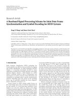
the major events leading to the development of fMRI are noted in Figure 1.1.
1937
1946
1956
1971
1975
1977
1989
1995
Isador Rabi measures the magnetic moment of the
nucleus of an atom.
Edward Purcell and Felix Bloch measure NMR in bulk
matter.
Ronald Bracewell uses a series of 1D strips to
reconstruct a 2D image with Fourier transform.
Raymond Damadian publishes evidence that NMR can
distinguish healthy from malignant tissue.
Paul Lauterbur extracts an image from NMR signals.
Richard Ernst introduces 2D NMR.
Damadian announces first whole body NMR scanner.
Mansfield introduces echoplanar MRI.
Seiji Ogawa introduces BOLD contrast agents in fMRI
MRI used clinically

fMRI used in brain mapping

Figure 1.1 Timeline of the development of fMRI.

In 1924, Wolfgang Pauli suggested that protons or neutrons (or both) move with
angular momentum and become magnetic under certain condition. In 1937, Isador
Rabi actually measured the magnetic moment of the nucleus, for which he called it
NMR. In the late 1960s, Raymond Damadian showed interest in the then controversial
theory of biologist Gilbert Ling, who argued that water in malignant cell differs in
organisation from water in healthy cell. He subsequently produced NMR spectra of

3
rats’ tumour in 1970, which showed different T1 and T2 readings for cancerous tissue
and healthy tissue. However, it is Paul Lauterbur, who succeeded in producing the
first NMR image in 1973, before Raymond Damadian, who subsequently produced
the first human NMR image in 1976. By the early 1980s, most MRI hardware had
been developed and the four theoretical contributions that explain why magnetic
resonance (MR) can produce images of the body’s interior were at hand. They are
namely, (i) Paul Lauterbur’s discovery that an image can be extracted for NMR using
single-line projection data – 1D MRI, (ii) Richard Ernst’s implementation of the
mathematics of Fourier transform that brought on data from 2D, (iii) Peter Mansfield
showed how practical imaging could be developed using echoplanar technique, that
leds to functional, or fast, magnetic resonance imaging a decade later, and (iv)
Raymond Damadian’s design for a practical whole body magnet capable for
performing imaging and spectroscopy.

Ordinary MRI data is acquired line by line, whereas echoplanar method acquires and
processes data from an entire plane at one time. This will be described in detail in
Section 2.1.6. Speed has the advantage of avoiding distortions caused by the motions
of breathing, heartbeats, blood flow, and intestinal moments, or movements of patient.

The initial breakthrough for fMRI came from Seiji Ogawa when he investigated the
radiofrequency (RF) signals when the brain functions [3]. He worked with the
knowledge that activated brain cells used more oxygen than cells at rest. The
deoxy-haemoglobin is paramagnetic and changes the magnetic field around it. This
distortion of the magnetic field, in turn, affects the magnetic resonance of nearby
water protons amplifying their signal as much as 10,000 times. Ogawa called this
effect blood oxygenation level dependent (BOLD) contrast imaging and published a

4
paper in 1990 [4]. The BOLD contrast image is exceptionally good when acquired
with magnet stronger than 4 Tesla. Ogawa’s discovery leads to the development of
effective fMRI.
1.1.2 Functional Magnetic Resonance Imaging
fMRI is a technique for localising brain activity. An fMRI machine is basically an
advance magnetic resonance imaging (MRI) machine that is programmed to detect a
functional signal rather than a structural signal. fMRI usually measures the blood
oxygenation level dependent (BOLD) signal on a voxel by voxel basis, which
increases with increased brain activity. With the availability of a functional scan, it is
possible to develop a method which can monitor a patient’s health continuously. This
is especially so in the case of a coma patient, where communication with the doctors
is not possible. The brain controls the whole body functions. Thus, a continuous
monitoring of the patient’s brain should tell a lot about the patient’s health.

Unfortunately, due to the cost of the equipment and shielding requirements, it is not
economical or practical to use fMRI for continuous monitoring. Furthermore, it is
technically impossible, as the BOLD signal will saturate under long exposure of a
constant strong magnetic field. Moreover, the use of RF pulses also restricts the
duration of scan on patients. Specific absorption rate (SAR) is the physiological
measure of the intensity of RF energy measured in Watts/kg (W/kg). Table 1.1 shows
the United States Food and Drug Administration (FDA) guideline on the safety

exposure limits on the RF and magnetic field [5].



5
Table 1.1
2
FDA guidelines on the safety limits
Type of exposure FDA limits
Static magnetic field 2 T
Magnetic Field
Transient magnetic field 3.0 T/s
Whole body 0.4 W/kg
1g of tissue 2.0 W/kg RF Field
Whole head 3.2 W/kg

Though fMRI has many advantages, due to the use of strong magnetic field, patients
with certain conditions cannot be scanned in the MRI machine. Cardiac pacemakers
and ferromagnetic metallic implants are known to be affected by the strong magnetic
field. The switches inside a cardiac pacemaker could become inoperative under a
static magnetic field of 0.2mT [6]. Ferromagnetic metallic implants, e.g. surgical clip,
could be twisted under the influence of the static magnetic field; this twisting effect
3

could cut vital blood vessels. Non-ferromagnetic metal implants can also cause
artefacts in MRI scans, rendering the scan useless if the implant is near the region of
interest. The strong magnetic field may also cause eddy currents in metallic implants
and devices, which may heat
4
up and might cause damage to the surrounding tissue.

Pregnant women are also advised against undergoing MRI scans, as the long term
effects of a strong magnetic field on the foetus are not well studied. These safety
aspects are well documented in [6] and usually discussed in various chapters of
standard MRI literature [5,7].



2
Table 1.1 is extracted from [5], Chapter 29.
3
Magnitude of twisting depends on several factors, like strength of static magnetic field, degree of
ferromagnetism, and size, shape and mass of the surgical clip [5].
4
The amount of heat generated depends on the MRI scan parameters and type of material used in the
implants or devices. However, this is rarely an issue because body heat loss mechanisms are very
efficient.

6
The principle of brain modularity states that different regions of the brain perform
different functions and hence measured brain signals should be able to decomposed
into their independent sources [8]. Independent component analysis (ICA) is a
powerful signal processing technique for blind source separation (BSS) which can
decompose mixed signals into their independent sources [9,10]. Therefore, ICA can
be applied to fMRI data for extracting the independent components. The fMRI signals
comprise effects from the applied stimulant, background activities (breathing,
heartbeat etc) and motion of patient etc. These effects are deemed to be independent
events, which could be separated using ICA. Linear ICA, because of its simplicity,
has been applied to fMRI brain signal data and has shown reasonably good results for
separating the brain’s activations due to stimulant from other causes (which are
considered as noise) [8].

However, EEG are widely accepted as nonlinear [11,12] and the BOLD signal has
also shown to be nonlinear [13,14]. This coincides with the balloon model, which
shows that the haemodynamic system is nonlinear [15]. The balloon model is a
biomechanical model of the haemodynamic system. Hence, a nonlinear algorithm
should be able to achieve a better decomposition of the fMRI data than a linear one.
1.2 Motivation
Currently, researchers especially in the medical field are using hybrid-techniques (e.g.
fMRI & EEG and fMRI & PET), where two or more different techniques are
combined to achieve better imaging qualities [16-18]. A hybrid method could prove to
be possible to achieve the desired continuous monitoring especially in an intensive
care unit environment. Electroencephalogram (EEG) is a well-established method to

7
understand the conditions of the brain using 1D/2D signal processing techniques. It
was suggested that it might be possible to combine the two techniques (fMRI with
EEG) [16,18] for better understanding of brain function. These two techniques
complement each other; fMRI has a high spatial but low temporal resolution, whereas
EEG has a low spatial but high temporal resolution. The hybrid scheme might then
result in high spatial and temporal resolution. Besides, EEG can be used for
continuous monitoring of the brain without any harmful effects to the patient. The
strategy is to use the high spatial resolution property of fMRI to map out the location
that generates the respective EEG signal. From there, it might be able to gauge the
health of the patient; perhaps even determine the state of coma and the chance of the
patient waking up from coma. This is especially so in view of the recent development
in brain computer interface (BCI) for completely paralysed patients [19].

From the background study, it is hypothesized that applying nonlinear ICA to the
fMRI signal data will result in better source separation of signals by their spatial
origin of fMRI signals than linear ICA algorithm. For this study, the PNL-ICA

algorithm was applied to fMRI signal data and the results was compared to that from
linear ICA algorithms for this application. This project is focused on the development
of nonlinear ICA algorithms.


8
CHAPTER 2
THEORY AND LITERATURE REVIEW

2.1 Magnetic Resonance Imaging
As the name implies, magnetic resonance imaging (MRI) makes use of resonance of
the atomic nucleus as signal for imaging. Atomic nuclei possess angular moment,
known as spin. This spin depends on the number of neutrons and protons in the
nucleus. Any nucleus with an even atomic mass number and even charge number has
no spin and hence has no nuclear magnetic resonance (MR) signal. Fortunately,
hydrogen-1, which has one of strongest spins, is relatively abundant in human body.
This section is mostly referenced from the book, “MRI – the basics” [20].

Magnetic susceptibility is the measure of how magnetised the substance is under a
magnetic field. Different substances have different degree of magnetisation; this
difference is the basis of image contrast in the MRI. There are three categories of
magnetic susceptibility commonly dealt with in MRI. They are diamagnetic,
paramagnetic and ferromagnetic. Diamagnetic substances have no unpaired electrons.
When place under an external magnetic field, B
0
, they have a weak induced magnetic
field, M, in the opposite direction to B
0
, thereby reducing the net magnetic field.
Paramagnetic substances have unpaired electrons. Under an external magnetic field,

B
0
, they produce an induced magnetic field, M, in the direction of B
0
, thereby
increasing the net magnetic field. Both diamagnetic and paramagnetic substances will
lose their magnetisation when the external magnetic field, B
0
, is removed. In contrast,
ferromagnetic substances retain their magnetisation even after the external field is
removed and are strongly attracted to the magnetic field.


9
In MRI, a constant magnetic field, B
0
, is applied to the patient. Then a RF pulse of a
specific frequency (resonance frequency of the tissue being examined) is directed at
the patient; this induces an oscillating magnetic field, B
1
, in the patient. The nuclei of
the tissue will be realigned due to the B
1
. After the RF pulse is removed, the nuclei
return to their original position, releasing a signal as they do so. This signal is
captured as the MR signal from the tissue. Figure 2.1 illustrate this basic concept of
MRI. Three orthogonal gradient coils are used to change the magnetic field’s
homogeneity applied to the patient. This is to allow spatial encoding of the received
signal.

Figure 2.1
5
Basic ideology of MRI
2.1.1 Larmor Frequency
In a magnetic field, the nucleus with a spin number, I, will have (2I + 1) discrete
energy levels [21]. Using hydrogen-1 as an example, it will have two energy states.
Hence, in a magnetic field, the hydrogen-1 nucleus will align either in parallel (lower
energy state) with the magnetic field or opposite (higher energy state) to it. However,
by applying a radiofrequency magnetic field, it is possible to attain a transition energy

5
Figure 2.1 is extracted from [20], Chapter 2.

10
state in between the highest and the lowest energy states. The Larmor equation,
Equation (2.1) below, shows this relationship.

γ
=
ω B (2.1)
where,
ω
is the Larmor frequency in MHz, γ is the gyromagnetic ratio in MHz/Telsa
and B is the magnetic field strength in Tesla. Table 2.1 shows the various properties
and relative abundance of nuclei found in the human body.
Table 2.1
6
Spin properties and natural abundance of various nuclei

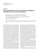
Without any external magnetic field, the proton only rotates about its own axis, as
shown in Figure 2.2(a). When a magnetic field, B
0
, is applied to the proton, besides
rotating about its own axis, it will also precess about the axis of the axis of B
0
, as
shown in Figure 2.2(b). Protons spin much faster along their own axis than around the
axis of
B
0
, that is, ω
spin
is much faster than ω
0
. ω
0
is the Larmor frequency
corresponding to
B
0
as shown in Equation (2.1).


6
Table 2.1 is extracted from [21], Chapter 3.
Nucleus

Natural Abundance
(%)
Spin
Frequency/Tesla
(MHz/T)
1
H 99.9 1/2 45.577
13
C 1.1 1/2 10.708
14
N 99.63 1 3.078
15
N 0.37 1/2 4.316
23
Na 100 3/2 11.268
19
F 100 1/2 40.007
31
P 100 1/2 17.254

11
spin
(a) (b)
B
0
spin

Figure 2.2 (a) A proton rotates about its own axis (b) When external magnetic field, B
0
, is applied, the

proton not only rotates about its own axis, but also rotates about the axis of B
0
.
2.1.2 Radio Frequency Pulse and Precession
Figure 2.3 illustrates the nuclei’s alignment at equilibrium (a) before and (b) after a
longitudinal magnetic field, B
0
, is applied to an ensemble of hydrogen-1 nuclei. As
seen in Figure 2.3(a), the nuclei are randomly aligned; thus there is no net
magnetisation. However, in Figure 2.3(b) when B
0
is applied to the ensemble of
nuclei, they align in parallel with this magnetic field. At equilibrium, a small majority
of the hydrogen-1 nuclei align in the direction of B
0
, thus forming a single net
magnetisation, M
0
in the direction of B
0
. Note that there is no net transverse magnetic
field perpendicular to B
0
, since the nuclei do not precess in phase with each other.

12

Figure 2.3 Illustration of the nuclei’s alignment at equilibrium (a) before and (b) after B
0
is applied

Figure 2.4(a) shows 3D coordinate system to depict the net magnetisation of the
system after B
0
was applied but before the RF pulse was transmitted. In Figure 2.4(b),
an RF pulse perpendicular to B
0
, is transmitted to the ensemble of nuclei. The RF
pulse, being an electromagnetic wave, will also have an oscillating magnetic field, B
1
,
perpendicular to B
0
. Note that the strength of B
0
(≥1T) is much greater than B
1

(~50mT). Figure 2.4(b) also shows the presence of transverse magnetic field, M
xy
,
and the flipping of net magnetisation
7
, M
net
, at an angle of
θ
away from z-axis. The
causes of flipping of M
net

and degree of flipping,
θ
, will be explained below.

7
Note that B
1
causes the flipping of the individual spins, M
net
flips because of the summation of these
individual spins. The text will refers these flippings of individual spins collectively as the flipping of
M
net
.