The application of ANFIS prediction models for thermal error compensation on CNC machine tools

Applied

Soft

Computing

27

(2015)

158–168
Contents

lists

available

at

ScienceDirect
Applied

Soft

Computing
j

ourna

l

ho

me

page:

www.elsevier.com/locate

/asoc
The

application

of

ANFIS

prediction

models

for

thermal

error
compensation

on

CNC

machine

tools
Ali

M.

Abdulshahed
∗
,

Andrew

P.

Longstaff,

Simon

Fletcher
Centre

for

Precision

Technologies,

University

of

Huddersfield,

HD1

3DH,

UK
a

r

t

i

c

l

e

i

n

f

o
Article

history:
Received

30

October

2012
Received

in

revised

form

14

October

2014
Accepted

13

November

2014
Available

online

21

November

2014
Keywords:
CNC

machine

tool
Thermal

error

modelling
ANFIS
Grey

system

theory
a

b

s

t

r

a

c

t
Thermal

errors

can

have

significant

effects

on

CNC

machine

tool

accuracy.

The

errors

come

from

thermal
deformations

of

the

machine

elements

caused

by

heat

sources

within

the

machine

structure

or

from
ambient

temperature

change.

The

effect

of

temperature

can

be

reduced

by

error

avoidance

or

numerical
compensation.

The

performance

of

a

thermal

error

compensation

system

essentially

depends

upon

the
accuracy

and

robustness

of

the

thermal

error

model

and

its

input

measurements.

This

paper

first

reviews
different

methods

of

designing

thermal

error

models,

before

concentrating

on

employing

an

adaptive
neuro

fuzzy

inference

system

(ANFIS)

to

design

two

thermal

prediction

models:

ANFIS

by

dividing

the

data
space

into

rectangular

sub-spaces

(ANFIS-Grid

model)

and

ANFIS

by

using

the

fuzzy

c-means

clustering
method

(ANFIS-FCM

model).

Grey

system

theory

is

used

to

obtain

the

influence

ranking

of

all

possible
temperature

sensors

on

the

thermal

response

of

the

machine

structure.

All

the

influence

weightings

of
the

thermal

sensors

are

clustered

into

groups

using

the

fuzzy

c-means

(FCM)

clustering

method,

the

groups

then

being

further

reduced

by

correlation

analysis.
A

study

of

a

small

CNC

milling

machine

is

used

to

provide

training

data

for

the

proposed

models

and
then

to

provide

independent

testing

data

sets.

The

results

of

the

study

show

that

the

ANFIS-FCM

model
is

superior

in

terms

of

the

accuracy

of

its

predictive

ability

with

the

benefit

of

fewer

rules.

The

residual
value

of

the

proposed

model

is

smaller

than

±4

␮m.

This

combined

methodology

can

provide

improved
accuracy

and

robustness

of

a

thermal

error

compensation

system.
©

2014

The

Authors.

Published

by

Elsevier

B.V.

This

is

an

open

access

article

under

the

CC

BY

license
(
/>1.

Introduction
Thermal

errors

of

machine

tools,

caused

by

internal

and

exter-
nal

heat

sources,

are

one

of

the

main

factors

affecting

CNC

machine
tool

accuracy.

Internal

heat

sources

comprise

all

heat

sources

that
are

directly

caused

by

the

machine

tool

and

cutting

process,

such
as

spindle

motors,

friction

in

bearings,

etc.

External

heat

sources
are

attributed

to

the

environment

in

which

the

machine

is

located,
such

as

neighbouring

machines,

opening/closing

of

machine

shop
doors,

cyclic

variation

of

the

environmental

temperature

during
the

day

and

night

and

differing

behaviour

between

seasons.

The
complex

thermal

behaviour

of

a

machine

is

created

by

interac-
tion

between

these

different

heat

sources.

According

to

various
publications

[1–3],

thermal

errors

represent

up

to

75%

of

the

total
positioning

error

of

the

CNC

machine

tool.

The

response

to

spindle
∗
Corresponding

author.

Tel.:

+44

0

1484

472596.
E-mail

addresses:

,

aa


(A.M.

Abdulshahed),



(A.P.

Longstaff),

s.fl
(S.

Fletcher).
heating

is

considered

to

be

the

major

error

component

among

them
[4]
.

One

of

the

methods

employed

to

avoid

this

problem

involves

the

use

of

thermally

stable

materials

such

as

fibre-reinforced

plas-
tics,

cement

concrete,

etc.

in

the

construction

of

the

machine

tool
or

to

design

symmetry

and

isolate

heat

sources

[4].

Although

these
are

good

practises

to

reduce

the

deformation

of

the

CNC

machine
tool

structure,

they

make

the

elimination

of

errors

very

expensive
and

can

lead

to

other

problems,

such

as

increased

vibration

or

lower
acceleration.
Another

technique

is

reducing

thermal

errors

through

numeri-
cal

compensation.

Compensation

is

a

process

where

the

thermal
error

present

at

a

particular

time

and

position

is

corrected
by

adjusting

the

position

of

a

machine’s

axes

by

an

amount
equal

to

the

error

at

that

position.

Error

compensations

can

be
more

attractive

than

making

physical

changes

to

the

machine
structure.

First,

error

compensation

is

often

less

expensive

than
the

design

effort,

manufacturing

and

running

costs

involved

in
error

avoidance.

Secondly,

error

compensation

is

more

adapt-
able

in

that

it

can

accommodate

changes

in

error

sources,
which

sometimes

cannot

be

accommodated

by

structural

change
techniques

[3].
/>1568-4946/©

2014

The

Authors.

Published

by

Elsevier

B.V.

This

is

an

open

access

article

under

the

CC

BY

license

( />A.M.

Abdulshahed

et

al.

/

Applied

Soft

Computing

27

(2015)

158–168

159
Many

compensation

techniques

have

been

explored

to

reduce
thermal

errors

in

a

direct

or

indirect

way.

Direct

compensation

is
simple

yet

efficient

philosophy,

making

use

of

directly

measured
displacements

between

a

tool

and

a

workpiece,

often

using

pro-
bing.

However,

direct

measurement

compensation

has

a

number
of

disadvantages.

For

instance,

it

is

likely

that

some

of

the

most
significant

thermal

problems

are

caused

by

rapid

thermal

changes.
Tracking

and

correcting

these

rapid

movements

would

require

fre-
quent

measurements.

When

a

tool-mounted

probe

is

used,

each
measurement

requires

a

break

in

machining,

therefore

introducing
unacceptable

time

delays.

In

addition,

probing

measurements

can
be

prone

to

errors

caused

by

swarf

or

coolant

on

the

surface

of

the

workpiece

[3].

This

can

be

overcome

by

repeated

measurements

or
other

means,

but

incurs

further

cost

in

terms

of

hardware

or

pro-
duction

time.

Realistically,

direct

thermal

compensation

is

most
applicable

to

fixed

tooling,

such

as

lathes

[2],

where

a

dedicated
sensor

can

be

conveniently

located.
1.1.

Thermal

modelling

methods
There

are

two

general

schools

of

thought

related

to

indirect
thermal

error

compensation.

The

first

method

uses

principle-based
models

such

as

the

finite

element

analysis

(FEA)

model

[5]

and

finite
difference

element

method

(FDEM)

[2].

Mian

et

al.

[5]

proposed
a

novel

offline

approach

to

modelling

the

environmental

thermal
error

of

machine

tools

in

order

to

reduce

the

downtime

required
to

calibrate

the

model.

Based

on

an

FEA

model,

the

method

was
found

to

reduce

the

machine

downtime

from

a

fortnight

to

12.5

h.
Their

modelling

approach

was

tested

and

validated

on

a

production
machine

tool

over

a

one-year

period

and

found

to

be

very

robust.
However,

building

a

numerical

model

can

be

a

great

challenge

due
to

problems

of

establishing

the

boundary

conditions

and

accurately
obtaining

the

characteristics

of

heat

transfer.
The

second

method

is

empirical

modelling

based

on

correlation
between

the

measured

temperature

changes

and

the

resultant

dis-
placement

of

the

functional

point

of

the

machine

tool,

which

is

the
change

in

relative

location

between

the

tool

and

workpiece.

Linear
regression

is

the

simplest

method

to

correlate

measured

tempera-
tures

with

resulting

displacement.

A

least

squares

approach

is

used
to

obtain

the

coefficients

that

determine

the

relationship

between
inputs

and

output

without

using

any

physical

equation.

Although
this

method

can

provide

reasonable

results

for

a

given

machine

test
regime,

the

thermal

displacement

usually

changes

with

variation
in

the

machining

process

and

the

environment,

which

introduces
and

error

into

the

model

[6].

The

linear

regression

model

is

also
time-consuming

and

labour

intensive

to

design.
In

recent

years,

it

has

been

shown

that

thermal

errors

can

be

suc-
cessfully

predicted

by

artificial

intelligence

modelling

techniques
such

as

artificial

neural

networks

ANNs

[7,8],

fuzzy

logic

[9],

adap-
tive

neuro-fuzzy

inference

systems

[8]

and

a

combination

of

several
different

modelling

methods

[10].
The

adaptive

neuro

fuzzy

inference

system

(ANFIS)

has

become
an

attractive,

powerful,

general

modelling

technique,

combining
well

established

learning

laws

of

ANNs

and

the

linguistic

trans-
parency

of

fuzzy

logic

theory

[11].

By

employing

the

ANN

technique
to

update

the

parameters

of

the

Takagi-Sugeno

type

inference

model,

the

ANFIS

is

given

the

ability

to

learn

from

training

data
in

the

same

way

as

an

ANN.

The

solutions

mapped

out

onto

a

fuzzy
inference

system

(FIS)

can

therefore

be

described

in

linguistic

labels
(fuzzy

sets)

[12].

Thus,

the

nodes

and

the

hidden

layers

are

deter-
mined

precisely

by

a

FIS

in

the

ANFIS

network.

This

eliminates
the

well-known

difficulty

of

determining

the

hidden

layer

of

ANN
models

and

at

the

same

time

improving

its

prediction

capability.
ANFIS

is

considered

because

it

does

not

require

complex

mathe-
matical

model,

it

is

fast

and

adaptive

and

the

developed

prediction
tool

can

be

implemented

quickly,

which

is

essential

for

thermal

errors

compensation.

ANFIS

techniques

have

already

been

applied
to

different

engineering

areas

such

as

support

to

decision-making
[13,14],

modelling

tool

wear

in

turning

process

[15],

and

mod-
elling

thermal

errors

in

machine

tools

[8,16].

Abdulshahed

et

al.

[8]
compared

the

ability

of

ANFIS

and

ANNs

to

predict

thermal

error
compensation

in

CNC

machine

tools.

The

results

indicated

that
although

ANNs

have

a

good

level

of

prediction

accuracy,

the

ANFIS
models

were

superior

in

terms

of

forecasting

ability.

Wang

[16]

also

proposed

a

thermal

model

using

ANFIS.

Experimental

results
indicated

that

the

thermal

error

compensation

model

could

reduce
the

thermal

error

to

less

than

9

␮m

under

cutting

conditions.

He
used

six

inputs

with

three

fuzzy

sets

per

input,

producing

a

com-
plete

rule

set

of

729

(3
6
)

rules

in

order

to

build

an

ANFIS

model.
Clearly,

Wang’s

model

is

practically

limited

to

low

dimensional
modelling.

It

is

important

to

note

that

an

effective

partition

of

the
input

space

can

decrease

the

number

of

rules

and

thus

increase

the
speed

in

both

learning

and

application

phases.

However,

a

reliable
and

reproducible

procedure

to

be

applied

in

a

practical

manner

in
ordinary

workshop

conditions

was

not

proposed.

For

example,

the
number

of

fuzzy

rules

increases

exponentially

when

the

number
of

variables

rises.

To

overcome

this

limitation,

fuzzy

c-means

algo-
rithms

could

be

used

to

determine

clusters

effectively,

providing
better

clustered

inputs

to

prediction

model.
1.2.

Reduction

of

model

inputs
Intuitively,

locating

a

large

number

of

sensors

on

a

machine
tool

structure

should

enhance

the

accuracy

of

the

thermal

error
model

since

it

increases

the

information

input.

However,

many
researchers

aim

to

reduce

the

number

of

required

temperature

sen-
sors.

Too

large

a

number

of

sensors

might

lead

to

an

increase

in

the
constraints

and

cost

of

the

compensation

system,

as

well

as

possibly
leading

to

poor

robustness

of

the

thermal

model

because

of

increase
in

data

noise.

Several

studies

have

used

statistical

approaches

such
as

engineering

judgement,

thermal

mode

analysis,

stepwise

regres-
sion

and

correlation

coefficients

to

select

the

temperature

sensors
for

thermal

error

compensation

models

[17].

Yan

and

Yang

[18]
proposed

an

MRA

model

combing

two

methods,

namely

the

direct
criterion

method

and

indirect

grouping

method;

both

methods

are
based

on

synthetic

Grey

correlation.

Using

this

method,

the

num-

ber

of

temperature

sensors

was

reduced

from

16

to

four

and

the
residual

range

was

reduced

for

69.1%.

Han

et

al.

[19]

proposed

a
correlation

coefficient

analysis

and

fuzzy

c-means

clustering

for
selecting

temperature

sensors

both

in

their

robust

regression

ther-
mal

error

model

and

ANN

model

[20];

the

number

of

thermal
sensors

was

reduced

from

32

to

five.

However,

these

methods

suf-

fer

from

the

following

drawbacks:

a

large

amount

of

data

is

needed
in

order

to

select

proper

sensors;

and

the

available

data

must

sat-
isfy

a

typical

distribution

such

as

normal

(or

Gaussian)

distribution
[21].

Therefore,

a

systematic

approach

is

still

needed

to

minimise
the

number

of

temperature

sensors

and

select

their

locations

so
that

the

downtime

and

resources

can

be

reduced

while

robustness
is

increased.
Grey

system

theory

is

a

method

introduced

by

Deng

in

early
1980s

[22]

with

the

intention

to

study

the

Grey

systems

by

using
mathematical

methods

with

poor

information

and

small

data

sets.
In

Grey

system

theory,

GM

(h,

N)

denotes

a

Grey

model,

where

h
is

the

order

of

difference

equation

and

N

is

the

number

of

vari-
ables.

The

GM

(h,

N)

model

can

be

used

to

describe

the

relationship
between

the

influencing

sequence

factors

and

the

major

sequence
factor

of

a

system.

Furthermore,

weights

of

each

factor

represent
their

importance

to

the

major

sequence

factor

of

the

system.

Its
most

significant

advantage

is

that

it

needs

only

a

small

amount

of
experimental

data

for

accurate

prediction,

and

the

requirement

for
the

data

distribution

is

also

low

[21].
160

A.M.

Abdulshahed

et

al.

/

Applied

Soft

Computing

27

(2015)

158–168
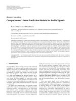
Fig.

1.

Basic

structure

of

ANFIS.
In

this

paper,

the

GM

(1,

N)

model

and

fuzzy

c-means

cluster-
ing

are

used

to

determine

the

major

sensors

influencing

thermal
errors

of

a

small

vertical

milling

machine

(VMC),

which

is

capa-
ble

of

simplifying

the

system

prediction

model.

Then

we

used

the
ANFIS

to

build

two

thermal

prediction

models

based

on

selected
sensors:

ANFIS

by

dividing

the

data

space

into

rectangular

sub-
spaces

(ANFIS-Grid)

and

ANFIS

by

using

fuzzy

c-means

clustering
method

with

ANFIS

(ANFIS-FCM).

This

combined

methodology

can
help

to

improve

robustness

of

the

proposed

model,

and

reduce

the
effect

of

sensor

uncertainty.
2.

Adaptive

neuro

fuzzy

inference

system

(ANFIS)

The

adaptive

neuro

fuzzy

inference

system

(ANFIS)

was
introduced

by

Jang

[11]
.

According

to

Jang,

the

ANFIS

is

a

neural
network

that

is

functionally

the

same

as

a

Takagi-Sugeno

type

infer-

ence

model.

ANFIS

has

become

an

attractive,

powerful

modelling
technique,

combining

well

established

learning

laws

of

ANNs

and
the

linguistic

transparency

of

fuzzy

logic

theory

within

the

frame-
work

of

adaptive

networks.

Fuzzy

inference

systems

(FIS)

are

one
of

the

most

well-known

applications

of

fuzzy

logic

theory.

In

the
fuzzy

inference

systems,

the

membership

functions

typically

have
to

be

manually

adjusted

by

trial

and

error.

The

FIS

model

performs
like

a

white

box,

meaning

that

the

model

designers

can

discover
how

the

model

achieved

its

goal.

On

the

other

hand,

artificial

neural
networks

(ANNs)

can

learn,

but

perform

like

a

black

box

regarding
how

the

goal

is

achieved.

Applying

the

ANN

technique

to

develop
the

parameters

of

a

fuzzy

model

allows

us

to

learn

from

a

given
set

of

training

data,

just

like

an

ANN.

At

the

same

time,

the

solu-
tion

mapped

out

into

the

fuzzy

model

can

be

explained

in

linguistic
terms

as

a

collection

of

“IF–THEN”

rules.
2.1.

ANFIS

architecture
The

architecture

of

ANFIS

is

shown

in

Fig.

1.

Five

layers

are

used
to

construct

this

model.

Each

layer

contains

several

nodes

described
by

the

node

function.

Adaptive

nodes,

denoted

by

squares,

rep-
resent

the

parameter

sets

that

are

adjustable

in

these

nodes.
Conversely,

fixed

nodes,

denoted

by

circles,

represent

the

param-
eter

sets

that

are

fixed

in

the

model.

Simple

ANFIS

architecture,
which

uses

two

variables

(T
1
and

T
2
)

as

inputs

and

one

output

(F:
thermal

drift),

will

be

described

in

this

section

in

order

to

explain

the

concept

of

the

ANFIS

structure.
Layer

1:

The

first

layer

is

the

fuzzy

layer

that

converts

the

inputs
into

a

fuzzy

set

by

means

of

membership

functions

(MFs).

It

con-
tains

adaptive

nodes

with

node

functions

described

as:
O
1,i
=


A
i
(T
1
),

for

i

=

1,

2
(1)
O
1,i
=


B
i−2
(T
2
),

for

i

=

3,

4

(2)
where

T

1
and

T
2
are

the

input

node

i,

A

and

B

are

the

linguis-
tic

labels

associated

with

this

node,

(T
1
)

and

(T
2
)

are

the
membership

functions

(MFs),

There

are

many

types

of

MFs

that
can

be

used.

However,

a

Gaussian

shaped

function

with

maximum
and

minimum

equal

to

1

and

0

is

usually

adapted.

Parameters

in
this

layer

are

defined

as

premise

parameters.
Layer

2:

Every

node

in

this

layer

is

a

fixed

node,

marked

by

a
circle

and

labelled

by

,

with

the

node

function

to

be

multiplied
by

input

signals

to

serve

as

output

signal.
O
2,i
=

w
i
=


A
i
(T
1
)

·


B
i−2

(T
2
),

for

i

=

1,

2

(3)
where

the

O
2,i
is

the

output

of

Layer

2.

The

output

signal

w
i
repre-
sents

the

firing

strength

of

the

rule.
Layer

3:

Every

node

in

this

layer

is

considered

a

fixed

node,
marked

by

a

circle

and

labelled

by

N,

with

node

function

to

nor-
malise

the

firing

strength

by

computing

the

ratio

of

the

ith

node
firing

strength

to

sum

of

all

rules’

firing

strength.
O
3,i
=
¯
w

=

w
i
w
1
+

w
2
,

for

i

=

1,

2

(4)
where

the

O
3,i
is

the

output

of

Layer

3.

The

quantity
¯
w is

known

as
the

normalised

firing

strength.
Layer

4:

Every

node

in

this

layer

is

an

adjustable

node,

marked
by

a

square,

with

node

function

as

following:
O
4,i
=
¯
w
i
·

f
i
,

for

i

=

1,

2

(5)
where

f
1

and

f
2
are

the

fuzzy

if–then

rules

as

follows:
•
Rule

1.

IF

T
1
is

A
1

and

T
2
is

B
1
,

THEN

f
1
=

p
1
T
1
+

q
1
T
2
+

r
1

•
Rule

2.

IF

T
1
is

A
2
and

T
2
is

B
2
,

THEN

f
2
=

p

2
T
1
+

q
2
T
2
+

r
2
where

p
i
,

q
i
and

r
i
are

the

parameters

set,

referred

to

as

the
consequent

parameters.
Layer

5:

Every

node

in

this

layer

is

a

fixed

node,

marked

also
by

a

circle

and

labelled

by

,

with

node

function

to

calculate

the
overall

output

by:
O
5,i
=

i
¯
w
i
·

f
i
=

i
w
i
f
i
w
i
=

f
out
=

Overall

output

(6)
The

simplest

learning

rule

of

ANFIS

is

“back-propagation”

which
computes

error

signals

recursively

from

the

output

layer

(Layer

5)
backward

to

the

input

nodes

(Layer

1).

This

learning

rule

is

exactly
the

same

as

the

back-propagation

learning

rule

used

in

the

common

feed-forward

neural

networks

[8,23].

Although

this

method

can

be
applied

to

identify

the

parameters

in

an

ANFIS

network,

the

method
is

generally

slow

and

likely

to

become

trapped

in

local

minima

[11].
Different

learning

techniques,

such

as

a

hybrid-learning

algorithm
[14]

or

genetic

algorithm

(GA)

[24],

can

be

adopted

to

solve

this
training

problem.

Better

performance

of

ANFIS

models

has

been
shown

by

adopting

a

rapid

hybrid

learning

method,

which

inte-
grates

the

gradient

descent

method

and

the

least-squares

method
to

optimise

parameters

[23,25,26].

Thus

in

this

paper,

the

hybrid
learning

method

is

used

for

constructing

the

proposed

models.
2.2.

Extraction

of

the

initial

fuzzy

model
In

order

to

start

the

modelling

process,

an

initial

fuzzy

model
has

to

be

derived.

This

model

is

required

to

select

the

input

vari-
ables,

input

space

partitioning

or

clustering,

choosing

the

number
and

type

of

membership

functions

for

inputs,

creating

fuzzy

rules,
and

their

premise

and

conclusion

parts.

For

a

given

dataset,

differ-
ent

ANFIS

models

can

be

constructed

using

different

identification
methods

such

as

grid

partitioning,

and

fuzzy

c-means

clustering
(FCM)

[23].
A

The

ANFIS-Grid

partition

method

is

the

combination

of

grid

partition

and

ANFIS.

The

data

space

divides

into

rectangular

sub-
spaces

using

axis-paralleled

partitions

based

on

a

pre-defined
A.M.

Abdulshahed

et

al.

/

Applied

Soft

Computing

27

(2015)

158–168

161
number

of

MFs

and

their

types

in

each

dimension

[27].

The

lim-
itation

of

this

method

is

that

the

number

of

rules

rises

rapidly
as

the

number

of

inputs

(sensors)

increases.

For

example,

if

the
number

of

input

sensors

is

n

and

the

partitioned

fuzzy

subset

for
each

input

sensor

is

m,

then

the

number

of

possible

fuzzy

rules
is

m
n
.

While

the

number

of

variables

raises,

the

number

of

fuzzy
rules

increases

exponentially,

which

requires

a

large

computer

memory.

According

to

Jang

[11],

grid

partition

is

only

suitable
for

problems

with

a

small

number

of

input

variables

(e.g.

fewer
than

6).

In

this

paper,

the

proposed

thermal

error

model

has

five
inputs.

It

is

reasonable

to

apply

the

ANFIS-Grid

partition

method.
B

The

ANFIS-fuzzy

c-means

clustering

is

the

most

common

method
of

fuzzy

clustering

[25].

Essentially,

it

works

with

the

principle

of
minimising

an

objective

function

that

defines

the

distance

from
any

given

data

point

to

a

cluster

centre.

This

distance

is

weighted
by

the

value

of

MFs

of

the

data

point

[25].

In

the

FCM

method,
which

is

proposed

to

improve

ANFIS

performance,

the

data

are
classified

into

pertinent

groups

based

on

their

degrees

of

MFs.

In
this

clustering

method,

it

is

assumed

that

the

number

of

clusters,
n
c
,

is

known

or

at

least

fixed.

It

divides

a

given

dataset

X

=

{x1,

.

.

.,
xn}

into

c

clusters.

More

detail

can

be

found

in

the

next

section.
In

order

to

obtain

a

small

number

of

fuzzy

rules,

a

fuzzy

rule
generation

technique

that

integrates

ANFIS

with

FCM

clustering
can

be

used,

where

the

FCM

is

used

to

systematically

identify

the
fuzzy

MFs

and

fuzzy

rule

base

for

ANFIS

model.

In

this

paper,

to
identify

premise

membership

functions,

the

two

aforementioned
methods

were

used

and

compared.
2.3.

Fuzzy

c-means

clustering
Fuzzy

c-means

(FCM)

is

a

soft

clustering

method

in

which

each

data

point

belongs

to

a

cluster,

with

a

degree

specified

by

a

mem-
bership

grade.

Dunn

introduced

this

algorithm

in

1973

[28]

and

it
was

improved

by

Bezdek

[29].

FCM

algorithm

is

the

fuzzy

mode
of

K-means

algorithm

and

it

does

not

consider

sharp

boundaries
between

the

clusters

[30,31].

Thus,

the

significant

advantage

of
FCM

is

the

allowance

of

partial

belongings

of

any

object

to

different
groups

of

the

universal

set

instead

of

belonging

to

a

single

group
totally.

FCM

partitions

a

collection

of

n

vectors

x
i
,

i

=

1,

2,

.

.

.,

n

into
fuzzy

groups,

and

determines

a

cluster

centre

for

each

group

such
that

the

objective

function

of

dissimilarity

measure

is

reduced.
i

=

1,

2,

.

.

.,

c

are

arbitrarily

selected

from

the

n

points.

The

steps
of

the

FCM

method

are

now

briefly

explained:

firstly,

the

centres

of
each

cluster

c
i
,

i

=

1,

2,

.

.

.,

c

are

randomly

selected

from

the

n

data
patterns

{x
1
,

x
2
,

x
3
,

.

.

.,

x
n
}.

Secondly,

the

membership

matrix

()
is

computed

with

the

following

equation:


ij
=
1

c
k=1
(d
ij
/d
kj
)
2/m−1
,

(7)
where,

ij
:

the

degree

of

membership

of

object

j

in

cluster

i;
M:

the

fuzziness

index

varying

in

the

range

[1,

∞];

and
d
ij
=

||c
i
−

x
j
||:

the

Euclidean

distance

between

c
i
and

x
j
.
Thirdly,

the

objective

function

is

calculated

with

the

following
equation.

The

process

is

stopped

if

it

falls

below

a

certain

threshold:
J(U,

c
1
,

c
2
,

.

.

.,

c
c
)

=
c


i=1
J
i
=
c

i=1
.
c

i=1

m
ij
d
2
ij
(8)
Finally,

the

new

c

fuzzy

cluster

centres

c
i
,

i

=

1,

2,

.

.

.,

c

are

cal-
culated

using

the

following

equation:
c
i
=

n
j=1

m
ij
x
j

n
j=1

m
ij
(9)
In

this

paper,

the

FCM

algorithm

will

be

used

to

separate

whole
training

data

pairs

into

several

subsets

(membership

functions)
with

different

centres.

Each

subset

will

be

trained

by

the

ANFIS,

as
proposed

by

Park

et

al.

[32].

Furthermore,

the

FCM

algorithm

will
be

used

to

find

the

optimal

temperature

data

clusters

for

thermal
error

compensation

models

[33].
3.

Selection

of

input

variables
A

large

number

of

thermal

sensors

may

have

a

negative
influence

on

predication

accuracy

and

robustness

of

a

thermal

pre-

diction

model.

One

of

the

difficult

issues

in

thermal

error

modelling
is

the

selection

of

appropriate

locations

for

the

temperature

sen-
sors,

which

is

a

key

factor

in

the

accuracy

of

the

thermal

error
model.

This

study

adopts

Grey

system

theory

to

identify

the

proper
sensor

positions

for

thermal

error

modelling.
The

Grey

systems

theory

is

a

methodology

that

focuses

on
studying

the

Grey

systems

by

using

mathematical

methods

with
a

only

few

data

sets

and

poor

information.

The

technique

works

on
uncertain

systems

that

have

partial

known

and

partial

unknown
information.

Its

most

significant

advantage

is

that

it

needs

a

small
amount

of

experimental

data

for

accurate

prediction,

and

the
requirement

for

the

data

distribution

is

also

low

[21].

There

are
many

types

of

Grey

models;

the

Grey

GM

(1,

N)

model

will

be

used
in

this

work.
3.1.

The

GM

(1,

N)

model
The

first-order

Grey

model,

GM

(1,

N),

is

a

multivariable

Grey
model

for

multi-factor

forecasting.

GM

(1,

N)

means

a

Grey

model
that

has

N

variables

including

one

dependent

variable

and

N

−

1
independent

variables.

Assume

that

there

are

N

variables,

x
i
(i

=

1,
2,

.

.

.,

N),

and

each

variable

has

n

initial

sequences

as:
x
(0)

i
=

{x
(0)
i
(1),

x
(0)
i
(2),

.

.

.,

x
(0)
i
(n)}

(i

=

1,

2,

.

.

.,

N)
First,

in

order

to

reduce

the

randomness

and

increase
the

smoothness

of

the

sequence,

the

accumulative

generation
operation

(AGO)

is

applied

to

convert

the

sequences

to

be

strictly

monotonic

increasing

sequences.

For

simplification,

let

us
define

the

first-order

accumulative

generation

operation

(1-AGO)
sequence

for

x
(0)
i
as:
x
(1)
i
=

{x
(1)
i
(1),

x
(1)
i
(2),

.

.

.,

x
(1)
i

(n)},
where,
x
(1)
i
(k)

=
k

j=1
x
(0)
i
(j)

(k

=

1,

2,

.

.

.,

n)
Then,

the

GM

(1,

N)

model

can

be

expressed

by

the

following
Grey

differential

equation

[21]:
x
(0)
1
(k)

+

az
(1)
1
(k)

=
N

j=2
b
j
X
(1)
j
(k)
=

b
2
x
(1)
2

(k)

+

b
3
x
(1)
3
(k)

+

·

·

·

+

b
N
x
(1)
N
(k),

(10)
162

A.M.

Abdulshahed

et

al.

/

Applied

Soft

Computing

27

(2015)

158–168
Fig.

2.

Block

diagram

of

the

proposed

system.
In

which,

z
(1)
1
(K)

is

defined

as:
z
(1)
1
(k)

=

0.5x
(1)

1
(k

−

1)

+

0.5x
(1)
1
(k)

k

=

2,

3,

4,

.

.

.,

n.
where

the

coefficients

a

and

b
j
are

called

the

system

development
parameter

and

the

driving

parameters,

respectively.
From

Eq.

(10),

we

can

write:
x
(0)
1
(2)

+

az
(1)
1
(2)

=

b
2

x
(1)
2
(2)

+

·

·

·

+

b
N
x
(1)
N
(2),
x
(0)
1
(3)

+

az
(1)

1
(3)

=

b
2
x
(1)
2
(3)

+

·

·

·

+

b
N
x
(1)
N
(3),
.
.

.
x
(0)
1
(n)

+

az
(1)
1
(n)

=

b
2
x
(1)
2
(n)

+

·

·

·

+

b
N
x
(1)
N
(n)
(11)
Eq.

(5)

can

be

written

in

the

matrix

form

as:
⎡
⎢

⎢
⎢
⎢
⎢
⎣
x
(0)
1
(2)
x
(0)
1
(3)
.
.
.
x
(0)
1
(n)
⎤
⎥
⎥
⎥
⎥
⎥
⎦
=
⎡
⎢

⎢
⎢
⎢
⎢
⎣
z
(1)
1
(2)

x
(1)
2
(2)

·

·

·

x
(1)
N
(2)
z
(1)
1
(3)

x
(1)
2
(3)

·

·

·

x
(1)
N
(3)
.
.
.
.
.
.
.
.
.
.
.
.
z
(1)
1

(n)

x
(1)
2
(n)

·

·

·

x
(1)
N
(n)
⎤
⎥
⎥
⎥
⎥
⎥
⎦
=
⎡
⎢
⎢
⎢
⎢

⎣
a
b
2
.
.
.
b
N
⎤
⎥
⎥
⎥
⎥
⎦
(12)
The

coefficients

of

the

model

can

then

be

obtained

using

the
least-square

estimate

method

as:
ˆ
Â

=

(B
T
B)
−1
B
T
Y,

(13)
where,
ˆ

 =
⎡
⎢
⎢
⎣
a
b
2
.
.
.
b
N
⎤
⎥
⎥
⎦
,

Y

=
⎡
⎢
⎢
⎢
⎣
x
(0)
1

(2)
x
(0)
1
(3)
.
.
.
x
(0)
1
(n)
⎤
⎥
⎥
⎥
⎦
,
B

=
⎡
⎢
⎢
⎢
⎣
z
(1)
1
(2) x

(1)
1
(2)

·

·

·

x
(1)
N
(2)
z
(1)
1
(3)

x
(1)
1
(3)

·

·

·

x
(1)
N
(3)
.
.
.
.
.
.
.
.
.
.
.
.
z
(1)
1
(n)

x
(1)
2
(n)

·

·

·

x
(1)
N
(n)
⎤
⎥
⎥
⎥
⎦
.
Therefore,

the

influence

ranking

from

the

independent

variables
to

the

dependent

variable

can

be

known

by

comparing

the

model
values

of

b
2
∼b
N
.
To

obtain

robust

models,

all

the

influence

weighting

of

thermal
sensors

is

clustered

into

groups

using

FCM.

Then,

one

sensor

from
each

cluster

is

selected

to

represent

the

temperature

sensors

of
the

same

category

according

to

its

influence

coefficient

with

the
Fig.

3.

Location

of

thermal

sensors

on

the

machine.
thermal

drift.

Therefore,

by

selecting

five

sensors,

the

ANFIS

models
can

be

built

easily

to

predict

the

thermal

drift.
The

whole

block

diagram

of

the

proposed

system

is

shown

in
Fig.

2,

where

variables

T1

to

TN

represent

the

temperature

data

cap-
tured

from

the

temperature

sensors,

and

the

thermal

drift

obtained
from

non-contact

displacement

transducers

(NCDTs).
4.

Experimental

work
4.1.

Setup

of

measurement

system
Fig.

3

shows

the

block

diagram

of

a

three-axis

vertical

milling
machine

(VMC).

The

motors

for

the

axes

are

directly

coupled

to

a
ballscrew

that

is

supported

by

bearings

at

each

end.

The

spindle

is
rotated

by

a

DC

motor

mounted

on

the

top

of

the

spindle

carrier.
The

spindle

speed

can

be

controlled

from

60

rpm

to

8000

rpm.

In
order

to

obtain

the

temperature

data

of

this

machine

tool,

a

total
of

76

thermal

sensors

are

placed

on

the

machine.

The

sensors

can
be

classified

into

different

categories

according

to

their

positions
as

illustrated

in

Table

1.
The

machine

tool

is

subjected

to

continuously

changing

oper-

ation

conditions.

It

is

rarely

maintained

at

steady

state

and

the
heat

generated

internally

will

vary

significantly

as

the

spindle

rota-
tion

speed

is

changed.

When

this

is

combined

with

the

effect

of
ambient

changes,

the

result

is

the

complex

thermal

behaviour

of
the

machine.

Five

non-contact

displacement

transducers

(NCDTs)
are

used

to

measure

the

displacement

of

a

precision

test

bar,
A.M.

Abdulshahed

et

al.

/

Applied

Soft

Computing

27

(2015)

158–168

163
0 10 20 30 40 50 60
0
5
10
15
Time (Minutes)
Temperature change (C)
°
Temperature sensor T11 (Test II, 4000 rpm)
Temperature sensor T11 (Test III, 4000 rpm)
Temperature sensor T11 (Test V, 8000 rpm)

Temperature sensor T11 (Test VI, 8000 rpm)
0 10 20 30 40 50 60
20
22
24
26
28
30
32
34
36
38
40
Time (Minutes)
Temperature (C
°
)
Temperature sensor T11 (Test II, 4000 rpm)
Temperature sensor T11 (Test III, 4000 rpm)
Temperature sensor T11 (Test V, 8000 rpm)
Temperature sensor T11 (Test VI, 8000 rpm)
(a) (b)
Fig.

4.

(a)

Absolute

temperature

of

the

selected

sensor

in

different

tests.

(b)

Magnitude

of

temperature

changes

in

different

tests.
Table

1
The

location

of

the

temperature

sensors.
Sensors

no.

Locations
1–7

Outside

the

column
8–32

Strip

1

Sensors

(placed

on

the

carrier)
33–61 Strip

2

Sensors

(placed

on

the

carrier)
62,63

Spindle

boss

64,65

Y

Scale

air
66,67

Y

bed

sensor
68

Column

air

top
69

Carrier

air
70

Table
71

Base

air
72

Spindle

air
73–75

Inside

the

column
76

Tool

air
representing

the

tool,

in

the

X,

Y

and

Z

axes.

The

configuration

is
shown

in

Fig.

3.
In

this

work,

a

variety

of

heating

and

cooling

tests

are

carried
out

in

different

ambient

conditions

and

different

spindle

speeds

of
the

VMC

(see

Table

2).

Brief

appraisal

of

the

methodology

shows
the

variation

considered

in

this

study.

Comparing

Test

I

and

Test

VI
shows

that

a

higher

spindle

rotation

speed

causes

a

larger

thermal
error

for

the

same

time

duration.

Whereas

comparing

Test

II

with
Test

III

and

Test

V

with

Test

VI,

it

can

be

seen

that

the

same

spindle
rotation

speed,

and

the

same

time

duration,

gave

rise

to

different
thermal

error.

This

was

due

to

change

of

the

ambient

conditions

and
hysteresis

effect.

More

detail

of

these

differences

can

be

observed
by

examining

a

selected

temperature

sensor

on

the

spindle

carrier
(T11);

Fig.

4(a)

shows

different

initial

conditions

of

the

machine

and
Fig.

4(b)

shows

the

different

magnitude

of

temperature

changes

in
different

tests.An

example

of

heating

and

cooling

test

is

illustrated
as

follows:

the

vertical

milling

machine

was

examined

by

running
at

its

highest

spindle

speed

of

8000

rpm

for

1

h

to

excite

the

largest
thermal

behaviour.

The

temperature

sensors

at

the

selected

points
0 20 40 60 80 100 120
-20

0
20
40
60
80
Time (Minutes)
Thermal displacement ( μm)
X axis
Y axis
Z axis
Fig.

5.

Thermal

drift

of

the

spindle

(spindle

speed

8000

rpm).
on

the

machine

tool

and

the

thermal

displacement

of

the

spindle

are
measured

simultaneously;

the

thermal

displacement

of

the

vertical
milling

machine

is

shown

in

Fig.

5.

The

maximum

displacement

of

the

X-axis

is

3

␮m,

the

Y-axis

is

79

␮m

and

the

Z-axis

is

22

␮m.

The
X-axis

thermal

displacement

is

much

smaller

than

that

of

the

Y-axis
and

the

Z-axis

due

to

the

mechanical

symmetry

of

the

machine

and
therefore

is

not

investigate

further

in

this

paper;

only

the

Y-axis

and
Z-axis

errors

are

considered.
4.2.

Influence

weighting

of

sensors

at

various

critical

points
The

selection

of

temperature

variables

is

a

key

factor

to

the

accu-
racy

of

the

thermal

error

model,

which

will

be

adversely

affected
Table

2
The

various

heating

and

cooling

tests.
Spindle

speed

(rpm)

Test

description

Total

time

(h)

Maximum

error
Y-direction

(␮m)
Test

name
4000

1

h

heating/1

h

cooling

2

25

Test

I
3

h

heating/2

h

cooling

5

35

Test

II
3

h

heating/2

h

cooling

5

40

Test

III
2

h

heating/1

h

cooling/2

h

heating/3

h

cooling

8

39

Test

IV
8000

1

h

heating/1

h

cooling

2

64

Test

V
1

h

heating/1

h

cooling

2

79

Test

VI
164

A.M.

Abdulshahed

et

al.

/

Applied

Soft

Computing

27

(2015)

158–168
Table

3
The

clustering

result.
GROUP

1

T18–T23,

T33–T53,

T72
GROUP

2

T24–T32,

T54–T61
GROUP

3

T8–T17,

T62,

T63
GROUP

4

T5,

T4,

T68,

T69,

T76

GROUP

5

T1–T3,

T6,

T7,

T64–T67,

T70,

T71,

T73–T75
if

there

is

insufficient

coverage

of

the

temperature

distribution.

At
the

same

time,

the

calibration/training

time

and

the

relative

cost
of

the

system

will

increase

if

the

number

of

input

variables

is

large.
Therefore,

the

location

of

suitable

temperature

sensors

should

be
determined

before

the

modelling

process.
By

applying

the

Grey

model

GM

(1,

N)

on

the

experimental
data

from

one

of

abovementioned

tests

(Test

VI),

the

influence
coefficients

can

be

obtained

as

follows:
Suppose

that

T1

∼

T76

represents

the

major

variables

(inputs)
x
(0)
2
∼x

(0)
n
and

the

measurement

of

the

NCDT

sensors

in

the
Y-direction

is

the

target

variable

(output)

x
(0)
1
.

The

influence
coefficients

can

be

obtained

by

Eq.

(13),

as


b
2



∼


b
76


.

The

greater
the

influence

weight,

the

greater

the

impact

on

the

thermal

error,
and

the

more

likely

it

is

that

the

temperature

variable

can

be
regarded

as

a

possible

modelling

variable.
Next,

the

influence

weightings

are

clustered

to

five

clusters

by
using

fuzzy

c-means

clustering

analysis

(see

Table

3).

Afterward,
one

sensor

from

each

cluster

is

selected

according

to

its

influence
weight

with

the

thermal

displacement

to

represent

the

tempera-
ture

sensors

of

the

same

category.

In

this

case

they

are

T18,

T55,

T63,
T68

and

T71.

These

temperature

sensors

are

located

on

the

spindle
carrier

(Strip

1

and

Strip

2),

spindle

boss,

ambient

near

the

column,
and

ambient

near

the

base,

respectively.
For

the

purpose

of

comparison,

another

test

was

carried

out

on
the

well-known

k-means

clustering.

The

soft

clustering

approach
produces

more

reasonable

results

than

the

hard

clustering.

How-
ever,

FCM

requires

more

iterations

than

k-means,

because

of

the
fuzzy

calculations.
4.3.

ANFIS

models

design
One

of

the

main

concerns

with

designing

a

thermal

error

com-
pensation

model

using

ANFIS,

or

any

other

self-learning

algorithm,
is

whether

the

training

data

that

was

measured

at

one

particular
operating

condition

of

the

CNC

machine

tool

would

be

sufficient
to

train

the

model

fully

for

other

operational

conditions.

In

other
words,

is

the

measured

data

sufficient

for

the

model

to

be

applicable
for

all

operating

conditions?
Ideally,

an

ANFIS

model

is

trained

by

a

training

set

that

includes
many

training

pairs

collected

from

all

likely

conditions.

However,
there

cost

of

machine

downtime

to

capture

the

training

data

is

a
significant

concern,

because

the

impact

on

productivity

can

have

a
high

penalty.

For

this

reason,

reducing

the

number

of

training

pairs
required

is

very

attractive.
Test

IV

was

considered

to

validate

the

method

of

reducing

the
number

of

training

cycles.

Measurements

of

thermal

error

and

cor-
responding

temperatures

were

recorded

while

the

machine

was
run

through

a

range

of

duty

cycle

as

follows:

It

was

allowed

to

run
at

spindle

speed

4000

rpm

for

120

min,

and

then

paused

for

60

min
before

running

for

another

120

min;

and

then

stopped

for

180

min.
Hence,

the

data

obtained

from

this

test

is

divided

into

three

parts
which

were

training,

checking,

and

testing

dataset.

The

checking
dataset

was

used

for

over-fitting

model

validation,

while

the

test-
ing

dataset

was

used

to

verify

the

accuracy

and

the

effectiveness

of
the

trained

model.
Five

temperature

sensors

from

Section

4.2

were

used

as

input
variables

to

the

models

and

the

thermal

displacement

in

the

Y-
direction

was

chosen

as

a

target

variable.

The

Gaussian

functions
Table

4
Performance

of

ANFIS-FCM

models

with

various

numbers

of

n
c
.
Models

Number

of
clusters

(n
c
)
Convergence
epochs
RMSE

of

testing
dataset
Model-1

2

200

2.3
Model-2

3

200

1.8
Model-3

4

100

1.7
Model-4

5

300

2.1
Model-5

6

200

5.6
Table

5

Linguistic

rules.
Linguistic

rules
1.

If

(T18

is

T18cluster1)

and

(T55

is

T55cluster1)

and

(T63

is

T63cluster1)

and
(T68

is

T68cluster1)

and

(T71

is

T71cluster1)

then

(out1

is

out1cluster1)
2.

If

(T18

is

T18cluster2)

and

(T55

is

T55cluster2)

and

(T63

is

T63cluster2)

and
(T68

is

T68cluster2)

and

(T71

is

T71cluster2)

then

(out1

is

out1cluster2)
3.

If

(T18

is

T18cluster3)

and

(T55

is

T55cluster3)

and

(T63

is

T63cluster3)

and
(T68

is

T68cluster3)

and

(T71

is

T71cluster3)

then

(out1

is

out1cluster3)

are

used

to

describe

the

membership

degree

of

these

inputs,

due

to
their

advantages

of

being

smooth

and

non-zero

at

each

point

[8].
After

setting

the

initial

parameter

values

in

the

ANFIS

models,

the
input

membership

functions

were

adjusted

using

a

hybrid

learning
scheme.
Extensive

simulations

were

conducted

to

determine

the

opti-
mum

structure

of

the

FIS

models

through

various

experiments.
The

optimal

number

of

MFs

was

determined

by

assigning

differ-
ent

numbers

of

MFs

for

the

ANFIS-Grid

model,

and

different

values
to

the

number

of

clusters

(n
c
)

for

the

ANFIS-FCM

model,

respec-
tively.

Too

few

MFs

will

not

allow

an

ANFIS

model

to

be

mapped
well.

However,

too

many

MFs

will

increase

the

difficulty

of

train-
ing

and

will

lead

to

over-fitting

or

memorising

undesirable

inputs
such

as

noise.

The

prediction

errors

were

measured

separately

for
each

model

using

the

root

mean

square

error

(RMSE)

index

with
the

testing

dataset.

An

example

of

selecting

the

optimum

structure
for

the

ANFIS-FCM

model

is

presented

as

follows:
In

this

modelling

method,

the

optimum

size

of

the

FIS

model

was
determined,

and

the

results

are

shown

in

Table

4.

Different

numbers
of

epochs

were

selected

for

each

model

because

the

training

process
only

needs

to

be

carried

out

until

the

errors

converge.

As

can

be
seen

in

Table

4,

it

cannot

simply

be

stated

that

better

results

will
be

obtained

with

more

clusters.

It

was

found

that

the

FIS

model
with

three

(n
c
=

3)

clusters

exhibited

the

lowest

RMSE

value

(1.7)

for

the

testing

dataset.

Consequently,

this

FIS

model

with

three

rules
was

considered

to

be

the

optimal.

The

corresponding

rules

of

the
optimum

model

are

provided

in

Table

5.
Similarly,

the

optimum

FIS

model

for

ANFIS-Grid

model

was
determined

by

arbitrarily

varying

the

number

of

MFs

from

2

to

4.
The

FIS

model

with

three

MFs

per

input

(243

rules)

was

found

to
be

the

optimum.
5.

Results

and

discussion
In

this

section,

the

aim

is

to

use

the

structure

of

the

ANFIS
models

described

in

the

previous

section

to

derive

a

thermal

error
compensation

system.

With

the

purpose

of

evaluating

the

pre-
diction

performance

of

the

models

generated

using

dataset

Test

IV,

the

remaining

datasets

Test

I,

Test

II,

Test

III,

Test

V,

and

Test
VI

were

used

to

run

the

models.

The

experimental

tests

were
carried

out

throughout

different

time

durations,

different

ambi-
ent

temperatures

and

different

spindle

rotation

speeds

in

order
to

validate

the

robustness

of

the

modelling

method.

The

perfor-
mance

of

the

models

used

in

this

study

was

computed

using

three
performance

criteria,

including

root-mean-square

error

(RMSE),
correlation

coefficient

(R
2
)

and

also

the

residual

value.

A.M.

Abdulshahed

et

al.

/

Applied

Soft

Computing

27

(2015)

158–168

165
0 20 40 60 80

100

120
-5
0

5
10
15
20
25
30
35
40
Time (Minutes)
Thermal displacement ( μm)
Thermal displacement (
μm)
ANFIS-FCM
Thermal Error
Residual value
0
20 40 60 80 100 120
-5
0
5
10
15
20
25
30
35
40
Time (Minutes)
ANFIS-GRID
Thermal Error

Residual value
Fig.

6.

(a)

ANFIS-Grid

model

output

vs

the

actual

thermal

drift.

(b)

ANFIS-FCM

model

output

vs

the

actual

thermal

drift

(2

h,

Test

I).
0 50

100

150

200

250

300
-5

0
5
10
15
20
25
30
35
40
Time (Minutes

)
ANFIS-FCM
Thermal Error
Residual value
0 50

100

150

200

250

300
-5
0
5
10

15
20
25
30
35
40
Time (Minutes)
Thermal displacement ( μm)
Thermal displacement (
μm)
ANFIS-GRID
Thermal Error
Residual value
Fig.

7.

ANFIS-Grid

model

output

vs

the

actual

thermal

drift.

(b)

ANFIS-FCM

model

output

vs

the

actual

thermal

drift

(5

h,

Test

II).
5.1.

Same

spindle

speed

under

different

operation

conditions
The

prediction

models

established

using

the

dataset

from

Test

IV

are

used

to

forecast

the

thermal

error

of

Test

I,

Test

II,

and

Test
III,

respectively.

In

all

experiments,

the

machine

was

examined

by
running

the

spindle

at

a

speed

of

4000

rpm,

but

the

duration

and
ambient

temperature

is

different

between

each

test

and

different

from

the

training

data,

as

illustrated

in

Table

2.

This

is

representa-
tive

of

a

machine

that

manufactures

similar

parts,

but

in

varying
factory

conditions.

The

temperature

sensors

at

the

selected

points
on

the

machine

tool

and

the

thermal

displacement

of

the

test

bar
are

measured

simultaneously.
0 50 100 150 200 250 300

-5
0
5
10
15
20
25
30
35
40
Time (Minutes)
ANFIS-FCM
Thermal Error
Residual value
0 50

100

150

200

250

300
-5
0
5
10
15

20
25
30
35
40
Time (Minutes)
Thermal displacement ( μm)
Thermal displacement (
μm)
ANFIS-GRID
Thermal Error
Residual value
Fig.

8.

ANFIS-Grid

model

output

vs

the

actual

thermal

drift.

(b)

ANFIS-FCM

model

vs

the

actual

thermal

drift

(5

h,

Test

III).
166

A.M.

Abdulshahed

et

al.

/

Applied

Soft

Computing

27

(2015)

158–168
0 20 40 60 80 100 120
0
10
20
30
40
50
60
70
Time (Minutes)
ANFIS-FCM
Thermal Error

Residual value
0 20 40 60 80

100

120
0
10
20
30
40
50
60
70
Time (Minutes)
Thermal displacement ( μm)
Thermal displacement ( μm)
ANFIS-GRID
Thermal Error
Residual value
Fig.

9.

ANFIS-Grid

model

output

vs

the

actual

thermal

drift.

(b)

ANFIS-FCM

model

output

vs

the

actual

thermal

drift

(5

h,

Test

V).
0

20

40

60

80

100

120

140
-10
0
10
20
30
40
50
60
70
80

Time (Minu

tes)
Thermal displacement (
μ
m)
ANFIS-GRID
Thermal Error
Residua

l value
0

20

40

60

80

100

120

140
-10
0
10
20

30
40
50
60
70
80
Time (Minutes)
Thermal displacement (μm)
ANFIS-FCM
Ther

mal Err

or
Residua

l value
Fig.

10.

ANFIS-Grid

model

output

vs

the

actual

thermal

drift.

(b)

ANFIS-FCM

model

output

vs

the

actual

thermal

drift

(5

h,

Test

VI).
Predictive

results

for

the

three

tests

using

ANFIS-Grid

model

and
ANFIS-FCM

model

are

shown

in

Figs.

6–8.

Results

show

that

these
two

models

are

competitive.

The

performance

of

each

of

the

two
thermal

prediction

models

is

presented

in

Table

6.

They

both

can
predict

the

new

observations

and

reduce

the

residual

value

to

less
than

±5

␮m

for

each

test.

It

is

clear

that

the

ANFIS-FCM

model

has
a

smaller

RMSE,

residual

value

and

higher

correlation

coefficient
than

the

ANFIS-Grid

model.
Table

6
Performance

calculation

of

the

used

models.
Test

name

Model

Number

of

rules

Performance

indices
R
2
RMSE

Residual

(␮m)
Test

I

ANFIS-Grid

model

243

0.96

1.53

±3
ANFIS-FCM

model

3

0.99

1.23

±2
Test

II

ANFIS-Grid

model

243

0.99

2.72

±4
ANFIS-FCM

model

3

0.99

0.57

±2
Test

III

ANFIS-Grid

model

243

0.98

2.78

±5
ANFIS-FCM

model

3

0.99

1.06

±2

Table

7
Performance

calculation

of

the

used

models.
Test

name

Model

Number

of

rules

Performance

indices
R

2
RMSE

Residual

(␮m)
Test

V

ANFIS-Grid

model

243

0.97

3.98

±8
ANFIS-FCM

model

3

0.99

2.78

±4
Test

VI

ANFIS-Grid

model

243

0.98

3.88

±7
ANFIS-FCM

model

3

0.99

2.78

±5
A.M.

Abdulshahed

et

al.

/

Applied

Soft

Computing

27

(2015)

158–168

167
5.2.

Different

spindle

speed

under

different

operation

conditions
The

prediction

models

established

using

the

dataset

from

Test
IV

were

further

tested

to

represent

a

machine

that

has

differ-
ent

manufacturing

parameters,

also

in

varying

factory

conditions.
The

machine

was

run

at

its

highest

spindle

speed

of

8000

rpm
for

one

hour

to

excite

more

thermal

response

than

during

the
training

data,

and

then

paused

for

another

hour

for

cooling

(see
Test

V

and

Test

VI).

Predictive

results

using

the

ANFIS-Grid

model
and

ANFIS-FCM

model

are

shown

in

Figs.

9

and

10.

The

evalu-
ation

criteria

values

are

provided

in

Table

7.

The

residual

error
obtained

using

the

ANFIS-FCM

model

was

again

better

than

the
ANFIS-Grid

model.

In

addition,

the

ANFIS-FCM

model

has

a

lower
RMSE

and

slightly

higher

correlation

coefficient

than

the

ANFIS-
Grid

model.

This

indicates

that

the

ANFIS-FCM

model

is

a

good
modelling

choice

for

predicting

the

thermal

error

of

the

machine
tools.
6.

Conclusions
This

paper

proposes

a

thermal

error

modelling

method

based
on

the

adaptive

neuro

fuzzy

inference

system

(ANFIS)

in

order
to

establish

the

relationship

between

the

thermal

errors

and

the
temperature

changes.

The

proposed

methodology

has

the

ability
to

provide

a

simple,

transparent

and

robust

thermal

error

com-
pensation

system.

It

has

the

advantages

of

fuzzy

logic

theory

and
the

learning

ability

of

the

artificial

neural

network

in

a

single
system.

The

optimal

locations

for

the

temperature

sensors

were
determined

through

the

Grey

model

and

fuzzy

c-means

cluster-
ing.

After

clustering

into

groups,

one

sensor

from

each

group

is
selected

according

to

its

influence

coefficient

value

with

the

ther-
mal

drift.

By

this

method,

the

number

of

temperature

sensors
was

reduced

from

76

possible

locations

to

five,

which

significantly
minimised

the

computational

time,

cost

and

effect

of

sensor

uncer-
tainty.
Two

types

of

ANFIS

model

have

been

discussed

in

this

paper:
using

grid-partitioning

and

using

fuzzy

c-means

clustering.

Both
models

were

constructed

and

tested

on

a

CNC

milling

machine.

The
results

from

the

two

sets

of

validation

tests

show

that

both

ANFIS-
based

models,

derived

from

a

single

heating-and-cooling

cycle,

can
improve

the

accuracy

of

the

machine

tool

by

over

80%

for

vary-
ing

ambient

conditions,

heating

durations

and

spindle

speeds.

The
ANFIC-FCM

produced

better

results,

achieving

up

to

94%

improve-
ment

in

error

with

a

maximum

residual

error

of

±4

␮m.

This
compares

favourably

with

other

compensation

methods

based
upon

parametric

or

self-learning

techniques,

such

as

similar

tests
by

the

authors

using

artificial

neural

networks

[8],

as

discussed

in
Section

1.
In

addition

to

the

better

absolute

accuracy,

the

ANFIS-FCM

has
been

shown

to

have

the

advantage

of

requiring

fewer

rules,

in

this
case

requiring

only

three

rules

as

opposed

to

the

243

found

to
be

optimal

for

the

ANFIS-Grid

model.

This

is

a

significant

benefit,
since

the

latter

method

is

significantly

more

laborious

to

con-
struct.
Therefore,

it

can

be

concluded

that

the

ANFIS-FCM

model

is
a

valid

and

promising

alternative

for

predicting

thermal

error

of
machine

tools

without

increasing

computation

overheads.
Acknowledgements
The

authors

gratefully

acknowledge

the

UK’s

Engineering

and
Physical

Sciences

Research

Council

(EPSRC)

funding

of

the

EPSRC
Centre

for

Innovative

Manufacturing

in

Advanced

Metrology

(Grant
Ref:

EP/I033424/1).
References
[1]

J.

Bryan,

International

status

of

thermal

error

research,

CIRP

Ann.

Manuf.

Tech-
nol.

39

(1990)

645–656.
[2]

J.

Mayr,

et

al.,

Thermal

issues

in

machine

tools,

CIRP

Ann.

Manuf.

Technol.

61

(2012)

771–791.
[3]

S.

Postlethwaite,

et

al.,

The

use

of

thermal

imaging,

temperature

and

distortion
models

for

machine

tool

thermal

error

reduction,

Proc.

Inst.

Mech.

Eng.

B:

J.
Eng.

Manuf.

212

(1998)

671–679.
[4]

R.

Ramesh,

et

al.,

Error

compensation

in

machine

tools

–

a

review:

Part

II.
Thermal

errors,

Int.

J.

Mach.

Tools

Manuf.

40

(2000)

1257–1284.
[5]

N.S.

Mian,

et

al.,

Efficient

estimation

by

FEA

of

machine

tool

distortion

due

to
environmental

temperature

perturbations,

Precis.

Eng.

37

(2013)

372–379.
[6]

B.

Tan,

et

al.,

A

thermal

error

model

for

large

machine

tools

that

considers

envi-
ronmental

thermal

hysteresis

effects,

Int.

J.

Mach.

Tools

Manuf.

82-83

(2014)
11–20.
[7]

J.

Chen,

et

al.,

Thermal

error

modelling

for

real-time

error

compensation,

Int.

J.
Adv.

Manuf.

Technol.

12

(1996)

266–275.
[8]

A.

Abdulshahed,

et

al.,

Comparative

study

of

ANN

and

ANFIS

prediction

models

for

thermal

error

compensation

on

CNC

machine

tools,

in:

Laser

Metrology

and
Machine

Performance

X,

Buckinghamshire,

2013,

pp.

79–88.
[9]

J H.

Lee,

et

al.,

Thermal

error

modeling

of

a

horizontal

machining

center

using
fuzzy

logic

strategy,

J.

Manuf.

Process.

3

(2001)

120–127.
[10]

A.

Abdulshahed,

et

al.,

Application

of

GNNMCI(1,

N)

to

environmental

thermal
error

modelling

of

CNC

machine

tools,

in:

Presented

at

the

the

3rd

Interna-
tional

Conference

on

Advanced

Manufacturing

Engineering

and

Technologies,
Stockholm,

2013,

pp.

253–262.

[11]

J.S.R.

Jang,

ANFIS:

adaptive-network-based

fuzzy

inference

system,

IEEE

Trans.
Syst.

Man

Cybern.

23

(1993)

665–685.

[12]

P.

Melin,

et

al.,

A

new

approach

for

time

series

prediction

using

ensembles

of
ANFIS

models,

Expert

Syst.

Appl.

39

(2012)

3494–3506.
[13]

G.

Özkan,

M.
˙
Inal,

Comparison

of

neural

network

application

for

fuzzy

and

ANFIS
approaches

for

multi-criteria

decision

making

problems,

Appl.

Soft

Comput.

24

(2014)

232–238.
[14]

S.

Kar,

et

al.,

Applications

of

neuro

fuzzy

systems:

a

brief

review

and

future
outline,

Appl.

Soft

Comput.

15

(2014)

243–259.
[15]

M.

Rizal,

et

al.,

Online

tool

wear

prediction

system

in

the

turning

process
using

an

adaptive

neuro-fuzzy

inference

system,

Appl.

Soft

Comput.

13

(2013)
1960–1968.
[16]

K.C.

Wang,

Thermal

error

modeling

of

a

machining

center

using

grey

system
theory

and

adaptive

network-based

fuzzy

inference

system,

in:

Cybernetics
and

Intelligent

Systems,

Bangkok,

2006,

pp.

1–6.
[17]

J.

Li,

et

al.,

Thermal-error

modeling

for

complex

physical

systems:

the-state-of-
arts

review,

Int.

J.

Adv.

Manuf.

Technol.

42

(2009)

168–179.
[18]

J.

Yan,

J.

Yang,

Application

of

synthetic

grey

correlation

theory

on

thermal

point
optimization

for

machine

tool

thermal

error

compensation,

Int.

J.

Adv.

Manuf.
Technol.

43

(2009)

1124–1132.
[19]

J.

Han,

et

al.,

Thermal

error

modeling

of

machine

tool

based

on

fuzzy

c-means
cluster

analysis

and

minimal-resource

allocating

networks,

Int.

J.

Adv.

Manuf.
Technol.

60

(2012)

463–472.
[20]

J.

Han,

et

al.,

A

new

thermal

error

modeling

method

for

CNC

machine

tools,

Int.
J.

Adv.

Manuf.

Technol.

(2012)

1–8.
[21]

S.

Liu,

et

al.,

Grey

Systems:

Theory

and

Applications,

vol.

68,

Springer,
Heidelberg,

2010.
[22]

J L.

Deng,

Control

problems

of

grey

systems,

Syst.

Control

Lett.

1

(1982)
288–294.
[23]

S.

Guillaume,

Designing

fuzzy

inference

systems

from

data:

an

interpretability-
oriented

review,

IEEE

Trans.

Fuzzy

Syst.

9

(2001)

426–443.
[24]

J.

Soto,

et

al.,

Time

series

prediction

using

ensembles

of

ANFIS

models

with
genetic

optimization

of

interval

type-2

and

type-1

fuzzy

integrators,

Int.

J.
Hybrid

Intell.

Syst.

11

(2014)

211–226.
[25]

A.

Karahoca,

D.

Karahoca,

GSM

churn

management

by

using

fuzzy

c-means
clustering

and

adaptive

neuro

fuzzy

inference

system,

Expert

Syst.

Appl.

38
(2011)

1814–1822.
[26]

J.

Soto,

et

al.,

A

new

approach

for

time

series

prediction

using

ensembles

of

ANFIS

models

with

interval

type-2

and

type-1

fuzzy

integrators,

in:

2013

IEEE
Conference

on

Computational

Intelligence

for

Financial

Engineering

&

Eco-
nomics

(CIFEr),

Singapore,

2013,

pp.

68–73.
[27]

M.

Wei,

et

al.,

Predicting

injection

profiles

using

ANFIS,

Inf.

Sci.

177

(2007)
4445–4461.
[28]

J.C.

Dunn,

A

fuzzy

relative

of

the

ISODATA

process

and

its

use

in

detecting
compact

well-separated

clusters,

J.

Cybern.

(1973).
[29]

J.C.

Bezdek,

Pattern

Recognition

with

Fuzzy

Objective

Function

Algorithms,
Kluwer

Academic

Publishers,

1981.
[30]

T.

Velmurugan,

Performance

based

analysis

between

k-means

and

fuzzy

c-
means

clustering

algorithms

for

connection

oriented

telecommunication

data,
Appl.

Soft

Comput.

19

(2014)

134–146.
[31]

A.K.

Jain,

Data

clustering:

50

years

beyond

k-means,

Pattern

Recognit.

Lett.

31
(2010)

651–666.
[32]

S.H.

Park,

et

al.,

Proceedings

of

2005

International

Symposium

on

Comparison
of

Recognition

Rates

Between

BP

and

ANFIS

with

FCM

Clustering

Method

on
Off-line

PD

Diagnosis

of

Defect

Models

of

Traction

Motor

Stator

Coil

in

Electrical
Insulating

Materials,

2005

(ISEIM

2005),

2005,

pp.

849–852.
[33]

S.M.N.

Arosha

Senanayake,

et

al.,

A

knowledge-based

intelligent

framework
for

anterior

cruciate

ligament

rehabilitation

monitoring,

Appl.

Soft

Comput.

20
(2014)

127–141.
168

A.M.

Abdulshahed

et

al.

/

Applied

Soft

Computing

27

(2015)

158–168
Ali

Mohmed

Abdulshahed

has

completed

his

five

year
bachelor

of

science

in

electrical

&

electronic

engineering
at

Sirt

University,

Brega-Libya.

Later

he

completed

his

MSc
in

engineering

control

systems

and

instrumentation

with
distinction

from

the

University

of

Huddersfield,

UK.

He
is

presently

working

in

the

field

of

artificial

intelligence
and

expert

systems.

He

is

now

a

PhD

student

in

the

Cen-
tre

for

Precision

Technologies

(CPT)

at

the

University

of
Huddersfield.
Andrew

Peter

Longstaff

is

a

Principal

Enterprise
Fellow

at

the

University

of

Huddersfield.

His

special-
ism

is

instrumentation,

measurement

data

acquisition,
data

processing

and

uncertainty

management

related
to

machine

tools,

robots

and

coordinate

measuring
machines.

In

the

past

sixteen

years

he

has

played

a

piv-
otal

role

in

both

government

and

industrially

sponsored
research

and

outreach

activities

in

the

field

of

manufac-
turing

accuracy

and

control.
Dr

Simon

Fletcher

is

a

Principal

Enterprise

Fellow

with
over

15

years’

experience

of

researching

and

teaching

in

the

field

of

Machine

Tool

Technology

with

particular

focus
on

metrology

and

advanced

design

techniques

for

preci-
sion

machining.

His

expertise

is

in

solid

modelling,

finite
element

analysis

and

mathematical

simulation

of

machin-
ing

errors.

Recently

he

has

worked

primarily

on

a

range

of
industrial

consultancy

projects

on

machine

tool

measure-
ment,

four

large

collaborative

European

funded

projects
and

has

over

60

publications.