Channel estimation and detection for multi input multi output (MIMO) systems
Bạn đang xem bản rút gọn của tài liệu. Xem và tải ngay bản đầy đủ của tài liệu tại đây (509.22 KB, 93 trang )
CHANNEL ESTIMATION AND DETECTION FOR
MULTI-INPUT MULTI-OUTPUT (MIMO) SYSTEMS
THI-NGA CAO
(B.Eng., HaNoi University of Technology)
A THESIS SUBMITTED
FOR THE DEGREE OF MASTER OF ENGINEERING
DEPARTMENT OF ELECTRICAL AND COMPUTER ENGINEERING
NATIONAL UNIVERSITY OF SINGAPORE
2006
SUMMARY
To meet the demand on very high data rates communication services, multiple
transmitting and multiple receiving antennas have been proposed for modern
wireless systems, where performance is limited by fading and noise. Most of
the current studies on multiple-input multiple-output (MIMO) systems assume
that the noise at receiving antennas are independent (white noise). In this
dissertation, we focus on MIMO systems under colored noise, i.e., the noise at
the receiving antennas are correlated.
Channel information estimation and data detection for MIMO systems under
spatially colored noise are studied. We propose an algorithm for pilot symbol
assisted joint estimation of the channel coefficients and noise covariance matrix. Our proposed method is applied in quasi-static flat fading, quasi-static
frequency selective fading and flat fast fading. A strategy to apply Sphere
Decoder in the spatially colored noise environment is also presented. This algorithm is used in the decoding stage of our proposed systems.
iii
ACKNOWLEDGEMENTS
I would like to express my sincere gratitude and appreciation to A/P Ng Chun
Sum, my supervisor, whose guidance, advice, patience are gratefully appreciated.
Special thanks also go to my colleague Mr. Zhang Qi for his fruitful and
enlightening discussions on various topics in communication theory.
iv
TABLE OF CONTENTS
Summary . . . . . . . . . . . . . . . . . . . . . . . . . . . . . . . . .
iii
Acknowledgements . . . . . . . . . . . . . . . . . . . . . . . . . . . .
iv
Table of Contents . . . . . . . . . . . . . . . . . . . . . . . . . . . . .
v
List of Figures . . . . . . . . . . . . . . . . . . . . . . . . . . . . . . .
vii
List of Symbols . . . . . . . . . . . . . . . . . . . . . . . . . . . . . .
1
1 Introduction
3
1.1
Motivations . . . . . . . . . . . . . . . . . . . . . . . . . . . . .
3
1.2
Contributions . . . . . . . . . . . . . . . . . . . . . . . . . . . .
5
1.3
Organization of the dissertation . . . . . . . . . . . . . . . . . .
6
2 Background
2.1
8
Continuous time MIMO system model . . . . . . . . . . . . . .
8
2.1.1
Transmitter structure . . . . . . . . . . . . . . . . . . . .
9
2.1.2
Fading channel model
. . . . . . . . . . . . . . . . . . .
10
2.1.3
Receiver structure . . . . . . . . . . . . . . . . . . . . . .
12
2.2
Discrete-time MIMO system model . . . . . . . . . . . . . . . .
13
2.3
Blocking and IBI Suppression for quasi-static frequency selective
2.4
fading channels . . . . . . . . . . . . . . . . . . . . . . . . . . .
16
Summary . . . . . . . . . . . . . . . . . . . . . . . . . . . . . .
19
3 Sphere Decoder
20
3.1
Introduction . . . . . . . . . . . . . . . . . . . . . . . . . . . . .
20
3.2
The Pohst and Schnorr-Euchner Enumerations . . . . . . . . . .
21
3.3
Sphere Decoders
. . . . . . . . . . . . . . . . . . . . . . . . . .
25
3.4
Application of Sphere Decoder in Communications Problems . .
27
3.5
Summary . . . . . . . . . . . . . . . . . . . . . . . . . . . . . .
33
4 Channel Estimation and Detection for MIMO systems
4.1
Decouple Maximum Likelihood (DEML) . . . . . . . . . . . . .
4.2
Channel estimation and Detection for quasi-static flat fading
34
34
channels . . . . . . . . . . . . . . . . . . . . . . . . . . . . . . .
36
4.2.1
System model . . . . . . . . . . . . . . . . . . . . . . . .
36
4.2.2
Channel estimation . . . . . . . . . . . . . . . . . . . . .
38
4.2.3
Symbol Detection . . . . . . . . . . . . . . . . . . . . . .
39
v
4.3
4.4
4.5
Channel estimation and detection for quasi-static frequency selective fading channels . . . . . . . . . . . . . . . . . . . . . . .
40
4.3.1
System model . . . . . . . . . . . . . . . . . . . . . . . .
40
4.3.2
Channel estimation . . . . . . . . . . . . . . . . . . . . .
44
4.3.3
Symbol Detection . . . . . . . . . . . . . . . . . . . . . .
44
Channel estimation and detection for flat fast fading channels .
46
4.4.1
Sytem model . . . . . . . . . . . . . . . . . . . . . . . .
46
4.4.2
Channel estimation . . . . . . . . . . . . . . . . . . . . .
49
4.4.3
Symbol detection . . . . . . . . . . . . . . . . . . . . . .
50
Summary . . . . . . . . . . . . . . . . . . . . . . . . . . . . . .
51
5 Results and Discussions
52
5.1
Quasi-static flat fading channels . . . . . . . . . . . . . . . . . .
53
5.2
Quasi-static frequency selective fading channels . . . . . . . . .
62
5.3
Flat fast fading channels . . . . . . . . . . . . . . . . . . . . . .
77
6 Conclusion and Recommendation
80
6.1
Conclusion . . . . . . . . . . . . . . . . . . . . . . . . . . . . . .
80
6.2
Recommendation . . . . . . . . . . . . . . . . . . . . . . . . . .
80
Bibliography
82
vi
LIST OF FIGURES
2.1
2.2
2.3
2.4
2.5
2.6
2.7
MIMO system model . . . . . . . . . . . . . . . . . . . . . . . .
QPSK signal mapping illustration . . . . . . . . . . . . . . . .
Spectrum shaping pulse blocks . . . . . . . . . . . . . . . . . .
The structure of received filters . . . . . . . . . . . . . . . . . .
The link from ith transmitter to j yh receiver . . . . . . . . . . .
Discrete MIMO system model . . . . . . . . . . . . . . . . . . .
(a) Block with P >> L. (b) General block transmission with
zero-padding . . . . . . . . . . . . . . . . . . . . . . . . . . . .
8
9
10
12
13
15
3.1
3.2
3.3
Geometrical interpretation of the integer least-squares problem.
Multiple antenna system . . . . . . . . . . . . . . . . . . . . . .
Frequency selective FIR channel . . . . . . . . . . . . . . . . .
21
29
30
4.1
4.2
4.3
Symbols structure for flat fading channels. . . . . . . . . . . . .
Symbols structure for frequency selective fading channels. . . .
Symbols structure for fast fading channels. . . . . . . . . . . . .
39
43
49
BER v.s. SNR for N = 44, M = 4, no LOS’s and in the colored
noise environment. . . . . . . . . . . . . . . . . . . . . . . . . .
5.2 BER v.s. SNR for N = 44, M = 4, no LOS’s and in the white
noise environment. . . . . . . . . . . . . . . . . . . . . . . . . .
5.3 BER v.s. SNR for N = 44, M = 4. Ricean factor of K = 2 and
in the colored noise environment. . . . . . . . . . . . . . . . . .
5.4 BER v.s. SNR for N = 44, M = 4. Ricean factor of K = 2 and
in the colored noise environment . . . . . . . . . . . . . . . . .
5.5 Average MSE of channel coefficients in 2 × 2 flat fading system,
N = 44 and M = 4, with and without LOS’s in the colored noise
environment. . . . . . . . . . . . . . . . . . . . . . . . . . . . .
5.6 Average MSE of channel coefficients in 2 × 2 flat fading system,
N = 44 and M = 4, with and without LOS’s in the white noise
environment. . . . . . . . . . . . . . . . . . . . . . . . . . . . .
5.7 Average MSE of elements of Σ in 2 × 2 flat fading system, N =
44 and M = 4, with and without LOS’s in the colored noise
environment. . . . . . . . . . . . . . . . . . . . . . . . . . . . .
5.8 Average MSE of elements of Σ in 2×2 flat fading system, N = 44
and M = 4, with and without LOS’s in the white noise environment . . . . . . . . . . . . . . . . . . . . . . . . . . . . . . . . .
5.9 BER v.s. SNR for the 2× 2 flat fading system, N = 44 and M =
4, without LOS’s in the colored and white noise environments. .
5.10 BER v.s. SNR for the 2 × 2 flat fading system, N = 44 and
M = 4, with LOS’s in the colored and white noise environments.
5.11 Compare the SN RM F B,i for 2 × 2 systems in the colored and
white noise environments. . . . . . . . . . . . . . . . . . . . . .
17
5.1
vii
53
54
55
56
57
57
58
58
59
59
61
5.12 Average MSE of each channel coefficients, without LOS paths,
in the colored noise environment. . . . . . . . . . . . . . . . . .
5.13 Average MSE of each channel coefficients, without LOS paths,
in the white noise environment. . . . . . . . . . . . . . . . . . .
5.14 Average MSE of elements of Σ, without LOS paths, in the colored noise environment. . . . . . . . . . . . . . . . . . . . . . .
5.15 Average MSE of elements of Σ, without LOS paths, in the white
noise environment. . . . . . . . . . . . . . . . . . . . . . . . . .
5.16 BER v.s. SNR for N = 44, M = 4, without LOS paths, in the
colored noise environment. . . . . . . . . . . . . . . . . . . . . .
5.17 BER v.s. SNR for N = 44, M = 4, without LOS paths, in the
white noise environment. . . . . . . . . . . . . . . . . . . . . .
5.18 BER v.s. SNR for N = 44, M = 4 and N = 24, M = 4, without
LOS paths, in the colored noise environment. . . . . . . . . . .
5.19 BER v.s. SNR for N = 44, M = 4 and N = 24, M = 4, without
LOS paths, in the white noise environment. . . . . . . . . . . .
5.20 BER v.s. SNR for N = 44, M = 4, without LOS paths, in the
colored and white noise environment. . . . . . . . . . . . . . . .
5.21 Average MSE of each channel taps. There exists LOS paths with
Rician factor of 5, in the colored noise environment. . . . . . .
5.22 Average MSE of each channel taps. There exists LOS paths with
Rician factor of 5, in the white noise environment. . . . . . . .
5.23 Average MSE of elements of Σ. There exists LOS paths with
Rician factor of 5, in the colored noise environment. . . . . . .
5.24 Average MSE of elements of Σ. There exists LOS paths with
Rician factor of 5, in the white noise environment. . . . . . . .
5.25 BER v.s. SNR for N = 44, M = 4, with LOS paths, in the
colored noise environment. . . . . . . . . . . . . . . . . . . . . .
5.26 BER v.s. SNR for N = 44, M = 4, with LOS paths, in the white
noise environment. . . . . . . . . . . . . . . . . . . . . . . . . .
5.27 Average MSE of each channel tap, with and without LOS paths,
in the colored noise environment. . . . . . . . . . . . . . . . . .
5.28 Average MSE of elements of Σ, with and without LOS paths, in
the colored noise environment. . . . . . . . . . . . . . . . . . .
5.29 Average MSE of each channel tap, with and without LOS paths,
in the white noise environment. . . . . . . . . . . . . . . . . . .
5.30 Average MSE of elements of Σ, with and without LOS paths, in
the white noise environment. . . . . . . . . . . . . . . . . . . .
5.31 BER v.s. SNR for N = 44, M = 4 and N = 24, M = 4, with
LOS paths, in the colored noise environment. . . . . . . . . . .
5.32 BER v.s. SNR for N = 44, M = 4 and N = 24, M = 4, with
LOS paths, in the white noise environment. . . . . . . . . . . .
5.33 BER v.s. SNR for N = 44, M = 4, with LOS paths, in the
colored and white noise environment. . . . . . . . . . . . . . . .
viii
63
63
64
64
65
65
66
67
68
69
69
70
70
71
72
72
73
73
74
75
75
76
5.34 BER v.s. SNR for fast fading channels in colored noise environment 78
5.35 BER v.s. SNR for fast fading channels in white noise environment. 79
ix
LIST OF SYMBOLS AND ABBREVIATIONS
C
R
Z
ZQ
∈
⊂
∅
{xn }+∞
n=−∞
ex or exp {x}
E {·}
Re(·)
Im(·)
log x
⊗
x1 (t) ∗ x2 (t)
|H|
N
i=1
N
i=1
x
x
x
∼
CN (m, σ 2 )
CN (m, Σ)
(·)T
(·)H
A†
0m×n
In
C
AWGN
BER
CIR
DEML
FIR
IBI
i.i.d.
ISI
LOS
set of complex numbers
set of real numbers
set of integer numbers
set of integer belong to set of [0, 1, 2, · · · , Q − 1]
is an element of
subset
empty set or null set
set of elements · · · , x−1 , x0 , x1 , · · ·
exponential function
(statistical) mean value or expected value
real part of a complex matrix/number
imaginary part of a complex matrix/number
natural logarithm of x
Kronecker product
convolution of x1 (t) and x2 (t)
determinant of matrix H
multiple product
multiple sum
ceiling function, the smallest integer greater than or equal x
floor function, the greatest integer less than or equal x
nearest integer to x
distributed according to (statistics)
complex Gaussian random variable with mean of m and
variance of σ 2
complex Gaussian random vector with mean of
m and covariance matrix of Σ
transpose of a matrix/vector
conjugate transpose of a matrix/vector
pseudo-inverse of a matrix A, A† = (AH A)−1 AH
zero matrix of size m × n
identity matrix of size n
QPSK symbols
Additive White Gaussian Noise
Bit-Error-Rate
Channel Impulse Response
Decouple Maximum Likelihood
Finite Impulse Response
Interblock Interference
independent and identical distributed
Intersymbol Interference
Line-Of-Sight
1
2
MIMO Multi-Input Multi-Output
MSE
Mean Square Error
PAM
Pulse Amplitude Modulation
QAM
Quadrature Amplitude Modulation
SD
Sphere Decoder
SNR
Signal-to-Noise Ratio
CHAPTER 1
INTRODUCTION
1.1
Motivations
Reliable communication over a wireless channel is a highly challenging problem
due to the complex propagation medium. The major impairments of the wireless
channel are fading and noise. Due to ground irregularities and typical wave
propagation phenomena such as diffraction, scattering, and reflection, when a
signal is launched into the wireless environment, it arrives at the receiver along
a number of distinct paths, referred to as multipath phenomenon. Each of these
paths has a distinct time-varying amplitude, phase and angle of arrival. These
multipaths add up constructively or destructively at the receiver. Hence, the
received signal can be distorted. The use of antenna arrays has been shown
to be an effective technique for mitigating the effects of fading and noise [1, 2,
3]. Antenna arrays can be employed at the transmitter, or receiver, or both
ends. With an antenna array at the receiver, fading can be reduced by diversity
techniques, i.e., combining independently faded signals on different antennas
that are separated sufficiently apart. If antennas receive independently faded
signals, it is unlikely that all signals undergo deep fades, hence, at least one
good signal can be received. To meet the requirement of very high data rates
for modern wireless networks, multiple antennas at both the transmitter and
receiver have been proposed [4, 5]. It was also proven that in a scattering rich
environment where channel links between different transmitters and receivers
fade independently, the Shannon’s information capacity of a MIMO channel
increases linearly with the smaller of the numbers of transmitting and receiving
3
4
antennas [6].
Most of the current studies on MIMO systems assume that the noise at the
receiving antennas are independent (white noise). However, in MIMO systems,
the noise may be dependent (colored noise) [7, 8]. In this dissertation, we focus
on MIMO systems under colored noise. Therefore, besides channel coefficients,
we have one more parameter to be concerned with, the noise covariance matrix. The ability to derive accurate information on channel properties from the
received signal is thus more challenging compared to that of an additive white
noise environment.
The design of suitable receiver structures that maximize system performance
is another vital task in communication systems. The Maximum-Likelihood
(ML) detector is well-known to be optimum but it has a major drawback of
requiring high computational complexity. Recently, a method to solve the ML
detection problems by using Sphere Decoders (SD), is proposed. Sphere decoders, in general, consisting of several variations, are algorithms derived from
the closest lattice point problem which is widely investigated in lattice theory
[9].
The SD was first applied to the ML detection problem in the early 90’s
[10] but gained main stream recognition with a later series of papers [11, 12].
To be specific, in [11], Viterbo and Boutros applied the SD to perform ML
decoding of multidimensional constellations in a single transmit antenna and
a single receive antenna system operating over an independent fading channel
with perfect channel state information at the receiver. The decoder performs a
bound distance search among the lattice points falling inside a sphere centered
at the received point. In [12], Oussama Damen et al. successfully applied the
5
SD in uncoded and coded multi-antenna systems. The historical background as
well as the current state of the art implementations of the algorithm have been
recently covered in two semi-tutorial papers [13] and [14].
From the day of appearance, the SD algorithm has found many applications.
Some examples include [12] which focuses on multi-antenna systems, [15] on the
CDMA scenario, and [16] where the sphere decoder is extended to generate soft
information required by concatenated coding schemes.
The complexity of SD is much lower than the directly implemented ML
detection method, which needs to search through all possible candidates before
making a decision. In [14], it is reported that the complexity of SD is polynomial
in m (roughly, O(m3 )) where m is the number of variables to be decoded. The
obtained performance of the SD algorithm is very promising. For example, in
[12], the authors apply SD to solve the detection problem in a MIMO system.
The results proved that SD can provide a huge performance improvement over
the well-known sub-optimal V-BLAST detection algorithm. Furthermore, the
complexity of SD method does not dependent on the number of signal points
in the signal constellations. SD also outperforms other suboptimal detection
scheme such as [17] in which authors applied the V-BLAST detection scheme
but in a new lattice where the basis is transformed to get a better orthogonality
among them in an operation called lattice reduction.
1.2
Contributions
In this dissertation, we consider MIMO systems under colored noise. We apply
the decouple maximum-likelihood (DEML) estimator, which was first used in
[18] to estimate the angle-of-arrival in antenna array systems, to estimate the
6
channel coefficients and noise covariance matrix for MIMO systems using pilot
symbols. Our method can be applied in quasi-static flat fading, quasi-static
frequency selective fading and flat fast fading.
A strategy for applying SD in colored noise environment is also introduced.
The improvement in the proposed system bit-error-rate (BER) performance, using SD as the detection algorithm and using the information from the proposed
channel estimation algorithm, over a classical detection method using perfect
channel information is shown by simulation.
1.3
Organization of the dissertation
Chapter 2 presents the continuous time MIMO system where the discrete
time MIMO system is developed.
Chapter 3 reviews the solution to the so-called closest lattice point problems
for the case of infinite lattice. The two strategies to solve the closest lattice point
problems, Pohst enumeration and Schnorr-Euchner enumeration, are presented.
This chapter also give some examples to show that in many communication
problems, the Maximum Likelihood (ML) problems can be translated into the
closest lattice point problems but in finite lattices. The Sphere Decoder, the
algorithm which solve the closest lattice point problems in finite lattice, is presented. Two Sphere Decoders are reviewed in the chapter, the first one relying
on the Pohst enumeration and the second one on Schnorr-Euchner enumeration.
The latter is noted to outperform the former in term of computational complexity. The Sphere Decoder so far deals with the case in which the noise at receivers
of MIMO systems are independent. This chapter also give a strategy to deal
with the case in which the noise components from receivers are correlated.
7
Chapter 4 presents the decouple maximum likelihood (DEML) estimator
to estimate the channel information for MIMO systems under three types of
fading: quasi-static flat fading, quasi-static frequency selective fading and flat
fast fading. The DEML estimator relies on the pilot symbols placed at the
beginning of the data frame to aid estimation of the channel coefficients and
the noise covariance matrix at the receiver. The application of Sphere Decoding
after obtaining the estimated channel information is presented.
Chapter 5 presents computer simulation results based on the theory developed in previous chapter.
Chapter 6 concludes the dissertation with the conclusion and recommendation for future works.
CHAPTER 2
BACKGROUND
In this chapter, we introduce the MIMO system model and the fading channel
model that are considered in this dissertation.
2.1
Continuous time MIMO system model
We consider a MIMO communication system equipped with Ni transmitters
and N0 receivers. The system under consideration is depicted in Figure 2.1.
Binary
Information
Source
b ( −1) b ( 0 ) b (1)
Signal
Mapping
✁
s
✂
s
(1)
( −1)
s
(2)
( −1)
s
(1)
(0)
s
(0)
s
(2)
(1)
(1) ✁
(2)
(1) ✂
Pulse
Shaping
Pulse
Shaping
.
.
.
✁
s
( Ni )
( −1)
s
( Ni )
(0)
s
( Ni )
(1) ✁
Pulse
Shaping
Received
Filter
✁ bˆ ( −1) bˆ ( 0 ) bˆ (1) ✁
Received
Filter
Decoding
.
.
.
.
.
.
Received
Filter
Channel
Information
Estimation
Figure 2.1: MIMO system model
8
9
2.1.1
Transmitter structure
Signal Mapping
In Figure 2.1, the binary information source generates the binary sequence
{b(k)}+∞
k=−∞ where k denotes the time index. This sequence is generated at
the bit rate of 1/Tb and consists of independent identically distributed binary
bits. The binary sequence is fed into the signal mapping block in which a bit
or a combination of bits is mapped onto a symbol for transmission. The outputs of the signal mapping blocks are denoted as {s(i) (k)}+∞
k=−∞ where superscript i, i = 1, 2, · · · , Ni denotes the ith transmitter. We consider a Gray-coded
quadrature phase-shift keying (QPSK) in which {00, 01, 11, 10} is mapped into
√
{1 + j, −1 + j, −1 − j, 1 − j} where j = −1 (see Figure 2.2). After the signal
mapping block, the symbol duration is T = 2 × Tb .
ℑ( s)
( 0,1)
−1
(1,1)
( 0, 0 )
1
1
−1
ℜ(s)
(1, 0 )
Figure 2.2: QPSK signal mapping illustration
Pulse shaping
The Ni parallel encoded sequences {s(i) (k)}+∞
k=−∞ , i = 1, 2, · · · , Ni are sent to
the pulse shaping blocks and transmitted simultaneously from Ni transmitters.
10
The pulse shaping blocks are illustrated in Figure 2.3 in which p(t) denotes its
impulse response.
s (1) ( t ) = ∑ s (1) ( k ) p ( t − kT )
✄ s(1) ( −1) s (1) ( 0 ) s (1) (1) ✄
k
p (t )
.
.
.
.
.
s(
☎ s ( Ni ) ( −1) s ( Ni ) ( 0 ) s ( Ni ) (1) ☎
p(t )
Ni )
( t ) = ∑ s ( N ) ( k ) p ( t − kT )
i
k
Figure 2.3: Spectrum shaping pulse blocks
The output of the ith pulse shaping block (corresponding to ith transmitter),
which are sent to ith transmitter for transmission, is written as
s(i) (t) =
k
2.1.2
s(i) (k)p(t − kT ), i = 1, 2, · · · , Ni .
(2.1)
Fading channel model
In urban area, fading is used to describe the rapid fluctuations of the amplitude
and phase in the received signal. Because of the short propagation distance (or
time), large-scale path loss may be ignored. Fading is caused by the interference
between two or more versions of transmitted signal which arrive at receiver
from different directions with different propagation delays. These multipath
signals, which come from reflections from the ground and surrounding structures
combine vectorially at the receiver, resulting in a received signal with randomly
distributed amplitude, phase, angle of arrival. Depending on the relationship
between signal parameters (such as bandwidth, symbol period, etc.) and the
channel parameters (such as delay spread and Doppler spread), the transmitted
11
signal will experience different types of fading [19, 20].
If the channel has a constant gain and linear phase response over a bandwidth which is greater than the bandwidth of the transmitted signal, then the
received signal undergoes flat fading. In flat fading, the multipath structure of
the channel is such that the spectral characteristics of the transmitted signal
are preserved at the receiver, i.e., all frequency components of the transmitted
signal are affected in the same manner by the channel. Flat fading is mainly experienced in narrow-band systems where the bandwidth of transmitted signal is
small compared with the coherence bandwidth of the channel, which is defined
as the reciprocal of the multipath delay spread of the channel. On the other
hand, if the channel possesses a constant gain and linear phase response over a
bandwidth that is smaller than the bandwidth of the transmitted signal, then
the channel introduces frequency selective fading on the received signal. Viewed
in the frequency domain, certain frequency components in the received signal
spectrum have greater gains than others. Frequency selective fading is mainly
experienced in broad-band systems where the the bandwidth of the transmitted
signal is larger than the coherence bandwidth of the channel. Frequency selective fading is manifested as time dispersion of the transmitted symbols within
the channel and thus induces ISI.
Depending on how rapidly the transmitted baseband signal changes as compared to the rate of change of the channel, a channel maybe classified as fast
fading or slow fading channel. In a fast fading channel, the channel impulse
response changes rapidly within the symbol duration. That is, the coherence
time of the channel is smaller than the symbol period of the transmitted signal. This causes frequency dispersion (also called time selective fading) due
12
to Doppler frequency shift, which leads to signal distortion. In a slow fading
channel, however, the channel impulse response changes at a rate much slower
than the transmitted baseband signal. Here, the coherence time is larger than
the symbol period of the transmitted signal.
In this dissertation, we will consider three types of fading: flat, frequency
selective and fast fading. The first two types of fading are considered in details
in the Section 2.2. The last type is considered in Section 4.4.
2.1.3
Receiver structure
At the receiver end, which is depicted in Figure 2.4, the received signal y (j) (t) at
the j th receivers, j = 1, 2, · · · , N0 , is a linear superposition of the Ni transmitted
signals from Ni transmitters perturbed by fading and additive Gaussian noise.
sampling at t = kT
y (1) ( t )
q (t )
.
.
.
.
y(
N0 )
(t )
y (1) ( n )
sampling at t = kT
q (t )
y(
N0 )
(n)
Figure 2.4: The structure of received filters
This received signal is sent to a received filter whose impulse response is
q(t) and the output of this filter is sampled with period of T . The obtained
discrete-time signals from all N0 receivers are used for the purpose of channel
information estimation and detection.
13
2.2
Discrete-time MIMO system model
To develop the discrete-time MIMO system model for the model in Figure 2.1,
we inspect only a link from ith transmitter to j th receiver in detail. This link is
illustrated in Figure 2.5.
Binary Information
Source
Signal
Mapping
x( j ) ( t )
Pulse Shaping
p (t )
Receiver filter
q (t )
( j)
w
(t )
s (i ) ( t )
Channel
c (i , j ) ( t )
sampling at t = kT
y( j) ( k )
y( j) (t )
additive white noise
Figure 2.5: The link from ith transmitter to j yh receiver
Let v(t) = p(t) ∗ c(i,j) (t). Then, v(t) becomes the modified transmitter filter
which includes the channel impulse response c(i,j) (t) of the link. The received
signal y (j) (t) after receiver filtering is written as
y (j) (t) =
(x(j) (τ ) + w(j) (τ ))q(t − τ )dτ
q(t − τ )
=
m
s(i) (m)
=
s(i) (m)v(τ − mT ) dτ +
q(t − τ )v(τ − mT )dτ +
m
q(t − τ )w(τ )dτ
q(t − τ )w(τ )dτ.
The sampled signal of y (j) (t) is given by
y (j) (k)
y (j) (t)
t=kT
s(i) (m)
=
m
= y (j) (kT )
q(kT − τ )v(τ − mT )dτ +w(j) (k)
=q(t)∗v(t)|t=(k−m)T
(2.2)
14
=
m
(j)
s(i) (m)h(i,j) (k − m) + w(j) (k)
q(nT − τ )w(τ )dτ and h(i,j) (k − m)
where w (k)
(2.3)
q(t) ∗ v(t)|t=(k−m)T .
The resulting received signal after sampling in the discrete time domain is
given by
y (j) (k) =
m
(i,j)
where h
s(i) (m)h(i,j) (k − m) + w(j) (k) = s(i) (k) ∗ h(i,j) (k) + w(j) (k) (2.4)
(k) is called the discrete time channel impulse response of the link.
From the investigation of one link, we generalized to our MIMO system with
Ni transmitter and N0 receivers to have the discrete-time MIMO system model
which is depicted in Figure 2.6.
th
In this model, the noise {w(j) (k)}+∞
receiver is assumed to
k=−∞ at the j
consist of i.i.d. Gaussian random variables with zero mean and variance of σw2
regardless of j. The noise at the N0 receivers, in general, are assumed to be
correlated.
The discrete-time channel impulse response of the link from ith transmitter
to j th receiver h(i,j) (k), i = 1, 2, · · · , Ni , j = 1, 2, · · · , N0 depends on the type
of fading under consideration.
If each link is a quasi-static frequency selective Rayleigh fading channel,
h(i,j) (k) is described by a linear, time-invariant finite impulse response as [20]:
l=L
(i,j)
h
(k) =
l=0
hi,j (l)δ(k − l); i = 1, 2, · · · , Ni , j = 1, 2, · · · , N0
(2.5)
where (L + 1) is the length of the channel impulse response, hi,j (l) is a complex
Gaussian random variable with zero mean and variance of σl2 , and δ(k) is the
Kronecker’s delta function.
If L = 0, then (2.5) specializes to the case of quasi-static flat fading where
h(i,j) (k) = hi,j (0)δ(k).
(2.6)
15
In this case we may simplify the notation by writing hi,j (0) = hi,j and
σ02 = σ 2 .
{s( ) ( k )}
1
∞
h(1,1) ( k )
k =−∞
∞
1
k =−∞
{s( ) ( k )}
2
{w( ) ( k )}
∞
h( 2,1) ( k )
k =−∞
{ y( ) ( k )}
∞
1
k =−∞
.
.
.
.
.
{s (
Ni )
( k )}k =−∞
∞
.
.
.
.
.
Ni ,1)
(k )
h(
1,N 0 )
(k )
h(
2, N0 )
(k )
h(
.
.
.
.
.
.
.
.
.
.
Ni , N0 )
N0 )
{
( k )}k =−∞
∞
}
y r( N0 ) ( k )
.
.
.
.
.
h(
{ w(
(k )
Figure 2.6: Discrete MIMO system model
∞
k =−∞
16
2.3
Blocking and IBI Suppression for quasi-static frequency selective fading channels
For transmission over wireless dispersive media, the channel induced ISI is a
major performance limiting factor. To mitigate such time-domain dispersive effect arising from frequency selectivity, it has been proven useful to transmit the
information-bearing symbols in blocks [21]. To be specific, we once again consider the link from the ith transmitter to j th receiver in our MIMO system without the presence of other links. This link is modeled as a quasi-static frequency
selective fading channel that has the length of CIR of (L+1). We group the serial
s(i) (k) into blocks of size P >> L and correspondingly define the mth transmitted block to be s(i) (m) = [s(i) (mP ) s(i) (mP + 1) · · · s(i) (mP + P − 1)]T and the
mth received block as y (j) (m) = [y (j) (mP ) y (j) (mP + 1) · · · y (j) (mP + P − 1)]T .
Using (2.4) and (2.5), we can relate transmit- with receive-block as (see Figure
2.7(a))
(i,j) (i)
y (j) (m) = H 0
(i,j) (i)
s (m) + H 1
s (m − 1) + w(j) (m)
(2.7)
where w(j) (m) is the corresponding noise vector, and the P × P matrices
(i,j)
Hl
, l = 0, 1 are defined as
(i,j)
H0
=
h (0)
0
0
i,j
..
.
hi,j (0)
0
...
hi,j (L) · · ·
..
...
···
.
0
···
hi,j (L)
···
0
···
0
..
.
···
...
0
· · · hi,j (0)
,
(2.8)