Simulation of a Multiple Input Multiple Output (MIMO) wireless system
Bạn đang xem bản rút gọn của tài liệu. Xem và tải ngay bản đầy đủ của tài liệu tại đây (1.45 MB, 73 trang )
DUBLIN CITY UNIVERSITY
SCHOOL OF ELECTRONIC ENGINEERING
Simulation of a Multiple Input Multiple Output
(MIMO) wireless system
John Fitzpatrick
TC4
52140938
April 2004
B.Eng
IN
Telecommunications Engineering
Supervised by Dr. Conor Brennan
Simulation of a MIMO wireless system – John Fitzpatrick
Acknowledgements
I would like to thank my supervisor Dr. Conor Brennan for his guidance, assistance and
approachability throughout this project. I would also like to thank John Diskin for his work
on the ray tracing program. Finally I would like to thank my parents and Laura for their
support throughout my project.
Declaration
I hereby declare that, except where otherwise indicated, this document is entirely my own
work and has not been submitted in whole or in part to any other university.
Signed: ...................................................................... Date: ...............................
ii
Simulation of a MIMO wireless system – John Fitzpatrick
Abstract
This project explores the development of a multiple input multiple output (MIMO) simulator
using ray tracing techniques. This project gives an overview of ray tracing techniques,
beamforming, MIMO channel models and MIMO systems. It explains the ability of MIMO
systems to offer significant capacity increases over traditional wireless systems, by
exploiting the phenomenon of multipath. By modelling high frequency radio waves as
travelling along localized linear trajectory paths, they can be approximated as rays, just as in
optics.
The radio environment is then represented using a ray tracing C++ program. I highlight
some of the different approaches used to realize a MIMO system, the most important being
the Singular Value Decomposition (SVD). I illustrate the development of the MIMO
simulator, through explanations of the techniques and algorithms I developed and used.
These algorithms model the system under ideal conditions with no noise distortions. I show
the use of the MIMO simulator created, and investigate the MIMO channel. The results
obtained show the affects of changing the different parameters of the system on the MIMO
channel and the radio environment.
Finally, in the conclusion, I discuss the future of MIMO systems and recommend further
modifications, which could be made to the MIMO simulator, to create a more accurate and
efficient system.
iii
Simulation of a MIMO wireless system – John Fitzpatrick
Table Of Contents
CHAPTER 1 - INTRODUCTION .......................................................................................1
CHAPTER 2 - TECHNICAL BACKGROUND.................................................................2
2.1
M
ULTIPATH
....................................................................................................................3
2.2
R
AY TRACING
.................................................................................................................3
2.3
B
EAMFORMING
...............................................................................................................4
2.4
L
INEAR ARRAYS
..............................................................................................................6
2.5
MIMO............................................................................................................................7
2.5.1 MIMO Transmission...............................................................................................8
2.5.2 The MIMO Channel H............................................................................................9
2.6
G
AUSSIAN
E
LIMINATION
...............................................................................................10
2.7
S
INGULAR
V
ALUE
D
ECOMPOSITION
(SVD)..................................................................12
CHAPTER 3 – IMPLEMENTATION OF RAY TRACING ..........................................13
3.1
R
AY TRACING
...............................................................................................................14
3.1.2 The ray tracing program ......................................................................................14
3.2
C
ONVERGENCE OF ORDER
.............................................................................................26
CHAPTER 4 - IMPLEMENTATION OF MIMO SIMULATOR..................................30
4.1
G
AUSSIAN
E
LIMINATION
...............................................................................................30
4.2
SVD ............................................................................................................................. 33
4.2.1 Operation of the SVD algorithm...........................................................................33
4.2.2 Matlab SVD ..........................................................................................................35
4.3
F
URTHER MODIFICATIONS TO THE RAY TRACING PROGRAM
..........................................39
4.4
P
LOTTING THE RESULTS
................................................................................................40
4.5
T
HE
MIMO
S
IMLATOR
.................................................................................................41
4.5.1 MIMO simulator users guide................................................................................43
CHAPTER 5 – RESULTS ..................................................................................................46
5.1
SVD
IN
F
REESPACE
......................................................................................................46
iv
5.2
N
UMBER OF ELEMENTS IN AN ARRAY
............................................................................49
Simulation of a MIMO wireless system – John Fitzpatrick
5.3
D
IELECTRIC PARAMETERS AND CORRIDOR MODEL
........................................................51
CHAPTER 6 - CONCLUSIONS AND FURTHER RESEARCH...................................55
Matlab code for Beamforming.......................................................................................58
C++ Gaussian Elimination Code..................................................................................60
Matlab Singular Value Decomposition (SVD) Code.....................................................64
Matlab ‘mimo’ Code...................................................................................................... 66
v
Simulation of a MIMO wireless system – John Fitzpatrick
Table of Figures
F
IGURE
2-1
M
ULTI
P
ATH
E
NVIRONMENT
........................................................................ 3
F
IGURE
2-2
SIMO
S
YSTEM
............................................................................................. 5
F
IGURE
2-3
L
INEAR
B
EAMFORMING
A
RRAY
................................................................... 6
F
IGURE
2-4
B
EAMFORMING
............................................................................................ 7
F
IGURE
2-5
T
HREE ELEMENT
MIMO
SYSTEM
................................................................. 8
F
IGURE
2-6
D
ATA TRANSMISSION IN
MIMO
SYSTEMS
................................................... 8
F
IGURE
3-1
B
UILDING
S
TRUCTURE
............................................................................... 15
F
IGURE
3-2
O
BLONG
(W
ALL
) ....................................................................................... 16
F
IGURE
3-3
F
ACE
.......................................................................................................... 17
F
IGURE
3-4
R
AY
N
ODES
............................................................................................... 19
F
IGURE
3-5
D
IRECT
R
AY
.............................................................................................. 20
F
IGURE
3-6
F
IRST
O
RDER
I
MAGE
.................................................................................. 21
F
IGURE
3-7
F
INDING
R
EFLECTION
P
OINTS
.................................................................... 22
F
IGURE
3-8
F
INDING THE REFLECTION POINT
................................................................ 25
F
IGURE
3-9
S
AMPLE POINTS FOR CONVERGENCE
.......................................................... 27
F
IGURE
3-10
C
ONVERGENCE GRAPH
,
B
LUE
=1
ST
,
RED
=2
ND
,
G
REEN
3
RD
O
RDER
........... 27
F
IGURE
3-11
2D
PLOT OF
4
TH ORDER ROOM WITH
6
WALLS
......................................... 28
F
IGURE
3-12
3D
PLOT OF
4
TH ORDER ROOM WITH
6
WALLS
......................................... 29
F
IGURE
4-1
S
CREENSHOT OF
G
AUSSIAN
E
LIMINATION PROGRAM
................................. 32
F
IGURE
4-2
S
CREENSHOT OF
C++
SVD
PROGRAM
....................................................... 34
F
IGURE
4-3
S
CREENSHOT OF RAY TRACING PROGRAM
.................................................. 43
F
IGURE
4-4
S
CREENSHOT
“P
LEASE ENTER
O
RDER
”...................................................... 43
F
IGURE
4-5
S
CREENSHOT
“P
LEASE RUN
‘
MYSVD
’
”...................................................... 44
F
IGURE
4-6
S
CREENSHOT
“P
LEASE RUN
‘
MIMO
’“......................................................... 44
F
IGURE
4-7
R
ESULT OF RAY TRACING PROGRAM
,
TX
ANTENNA IN FREESPACE
............. 45
F
IGURE
4-8
R
ESULT OF RAY TRACING PROGRAM
,
RX
ANTENNA IN FREESPACE
............ 45
F
IGURE
5-1
TX
FREESPACE ANTENNA GAIN PLOT
......................................................... 46
F
IGURE
5-2
RX
FREESPACE ANTENNA GAIN PLOT
......................................................... 47
F
IGURE
5-3
TX
FREESPACE ANTENNA GAIN PLOT WITH ANTENNA SHIFTED UP
............. 48
F
IGURE
5-4
RX
FREESPACE ANTENNA GAIN PLOT WITH ANTENNA SHIFTED UP
............. 48
F
IGURE
5-5
3
ELEMENT ANTENNA ARRAY
..................................................................... 49
F
IGURE
5-6
5
ELEMENT ANTENNA ARRAY
..................................................................... 50
F
IGURE
5-7
7
ELEMENT ANTENNA ARRAY
..................................................................... 50
F
IGURE
5-8
TX
CORRIDOR MODEL
................................................................................ 52
F
IGURE
5-9
RX
CORRIDOR MODEL
................................................................................ 52
vi
Simulation of a MIMO wireless system – John Fitzpatrick
F
IGURE
5-10
TX
CORRIDOR MODEL
,
INCREASED DIELECTRIC PARAMETERS
................. 53
F
IGURE
5-11
RX
CORRIDOR MODEL
,
INCREASED DIELECTRIC PARAMETERS
................. 54
vii
Simulation of a MIMO wireless system – John Fitzpatrick
Chapter 1 - Introduction
In the modern era of communications, the ability to send large volumes of data is crucial.
With the increasing use of wireless LAN technology and third generation mobile telephony
systems, the demand for data services has never been greater. The bandwidth of wireless
communication systems is often limited by the cost of the radio spectrum required. Any
increase in bit rate, which can be realised without increasing the bandwidth, makes the
system more spectrally efficient and less costly. Traditional wireless communication
systems have been made more spectrally efficient through the use of clever coding
techniques and algorithms. However, the fundamental bandwidth limitation does not change.
Multiple Input Multiple Output (MIMO) communication systems have been an increasingly
hot topic of research over the past eight years, due to their ability to greatly increase spectral
efficiencies.
As opposed to traditional wireless systems, in which there is one transmitting and one
receiving antenna, MIMO systems use arrays of multiple antennas at both ends of the
communication link, all operating at the same frequency at the same time. This introduces
spatial diversity into the system, which can be used to tackle the problem of multipath. In
wireless communications system, such as point to point radio links, radio waves do not
simply propagate from the transmit antenna to the receive antenna. Rather they bounce and
scatter off objects, this effect is known as multipath. This effect is regarded as an
impediment to the accurate transmission of data in traditional wireless links. MIMO systems
exploit multipath by using the rich scattering environment to increase the spectral efficiency
of the wireless system.
The modelling of radio waves on a large scale can be very complex. There is however, a
simplification. At high frequencies radio waves can be approximated as travelling along
localized paths. This is similar to the geometrical treatment of light rays in optics. Using ray
tracing methods, complex radio environments can be modelled.
The use of numerical techniques is crucial to the operation of MIMO systems. Algorithms
and signal processing at both ends of a MIMO wireless link are crucial to encode and
1
Simulation of a MIMO wireless system – John Fitzpatrick
decode the data. The most important numerical method in MIMO systems is Singular Value
Decomposition (SVD). This allows the complex path, which exists between transmitter and
receiver to be analysed and simplified.
By combining the above techniques it was the aim of this project to develop a fully
operational MIMO simulator. The simulator needed to model indoor radio environments and
be easy to use.
Chapter 2 - Technical Background
2
Simulation of a MIMO wireless system – John Fitzpatrick
In wireless communications system, such as point to point radio links, radio waves do not
simply propagate from the transmit antenna to the receive antenna. Rather they bounce and
scatter off objects. This effect is known as multipath. When the radio waves strike an object
in the environment, they scatter randomly as can be seen in figure 2.1. This is also known as
independent Rayleigh scattering. The red line shows the direct propagation path, whereas
the many blue lines show the multiple propagation paths produced by multipath.
Figure 2-1 MultiPath Environment
2.1 Multipath
Multipath results in multiple copies of the same transmitted signal arriving at the receiver, at
different times. As they arrive at different times they have varying phase delays, which can
result in scattered signals combining destructively at the receiver producing destructive
interference and fading. To carry out any simulation, the multipath environment needs to be
modelled. This is done using ray tracing.
2.2 Ray tracing
The radio environment was modelled using ray tracing. Ray tracing was initially developed
in the field of computer graphics to produce photorealistic computer generated images. Ray
tracing operates by calculating the path taken by a ray of light from a light source to the
point of interest. At frequencies greater than approximately 900MHz, radio waves can be
described as travelling along localized ray paths (i.e. approximately a straight line). The
3
Simulation of a MIMO wireless system – John Fitzpatrick
reasoning behind treating the waves as having linear trajectories stems from Maxwell’s
equations.
At high frequencies a more simple method can be used for handling electromagnetics. These
are known as asymptotic methods, more specifically Lumberg-Kline asymptotic expansions.
These are methods of simplification for the solution to Maxwell’s equations.
∑
∞
=
−
≈
0
)(
)(
)(
),(
n
n
n
rjf
j
rH
erH
ω
ω
ψ
∑
∞
=
−
≈
0
)(
)(
)(
),(
n
n
n
rjf
j
rE
erE
ω
ω
ψ
Most of the variables in these equations such as the phase function part are of very
complicated and I did not delve into their origin. Asymptotic methods are methods for
expanding functions, evaluating integrals, and solving differential equations, which become
increasingly accurate as some parameter approaches a limiting value [12]. The term of
interest is the frequency term
ω
. As the frequency approaches zero, only the first term of
the summation of both the electric field and magnetic field remain. This first term is called
the geometrical optics field as it encompasses the classical geometric optics field
characteristics [12]. Using the first term, the geometrical optics field, it can be shown how it
behaves as a ray, which is infinitesimal in width. I did not go into any more detail on this but
for further information please see the noted reference.
For this reason ray tracing can be used as a method for the simulation and approximation of
radio wave propagation at high frequencies. The ray tracing of radio waves operates in the
same manner as optical ray tracing, where transmitters replace light sources and the points
of interest are the receivers.
2.3 Beamforming
One solution to the problem of Multipath is to use directional antennas with a single antenna
at either end. Though these will only work if both ends of the link are static, if the receiver
or transmitter is mobile then motor driven directional antennas to rotate the transmitter can
4
Simulation of a MIMO wireless system – John Fitzpatrick
be used. However this is not very practical on a small scale. Another solution is to use
multiple antennas at either the transmitting or receiving end of a link, to accomplish what is
known as beamforming. Beamforming techniques were originally developed for
applications in radar and sonar systems. Using multiple antennas introduces spatial diversity
into the system. These antennas are also known as ‘smart antennas’. Spatial diversity is
based upon the fact that two signals detached in space exhibit independent fading in the
radio channel [3].
Figure 2.2 below, shows a smart antenna system with multiple antennas at one end of the
link. These systems are also known as SIMO (single-input multiple output). Originally
multiple antennas were placed at the receivers to introduce spatial diversity. This proved to
be too costly and inefficient and the multiple antennas were then placed at the transmitters.
Figure 2-2 SIMO System
Figure 2.2 above, shows a SIMO system operating in a simple modelled room with six
walls. In this case there is one transmitting antenna and three receive antennas. The idea
behind this system is that the probability of not being able to successfully detect a signal,
due to destructive interference, decreases exponentially with the number of antennas used in
a linear array.
5
Simulation of a MIMO wireless system – John Fitzpatrick
2.4 Linear arrays
Beamforming can be accomplished by using many different types of arrays, such as linear,
circular and planar arrays. I will only be considering linear arrays as shown in figure 2.3.
The principal behind beamforming is to introduce different power and phase weightings to
each of the antennas in the array. This is done in such a way as to generate constructive
interference in the desired direction.
Figure 2-3 Linear Beamforming Array
A linear array is shown in figure 2.3, the elements are uniformly spaced with spacing d. It
shows a wave incident on the array at an angle
θ
, with respect to the normal. The wave
arrives earlier at element 2 than at element 0 or 1. The distance between each element is
given by
θ
sind
, and therefore the phase delay between two adjacent elements will be the
time it takes the incident wave to travel the extra distance. The spacing between the
elements must be large enough so as to achieve independent fading. If they are not
appropriately spaced, there will be a loss in spatial diversity.
When different phase and power weightings are applied to transmitting linear arrays,
beamforming can be produced. The average signal-to-noise ratio (SNR) is increased using
beamforming, by focusing energy in desired directions; this is shown in figure 2.4.
6
Simulation of a MIMO wireless system – John Fitzpatrick
Figure 2-4 Beamforming
As is seen in the above figure, the different applied weightings result in destructive and
constructive interference in such a way so as to create a main lobe of constructive
interference in a particular direction, this is known as the directivity. This plot was obtained
using the Matlab code in appendix 1. This effect can also be implemented at the receiver end
of a link by phasing and weighting the received signals. However, in severe multipath
environments, beamforming will no longer be effective, as the signals are too severely
scattered to be effectively recovered.
2.5 MIMO
MIMO exploits multipath, traditionally a pitfall in wireless communications, to enhance
rather than degrade the signal. MIMO systems consist of multiple transmitters and multiple
receivers. For MIMO systems to be most effective, a rich multipath scattering environment
is needed to create independent propagation channels. It is the rich scattering in the
propagation channel, which offers multiple parallel sub channels at the same frequency,
therefore giving higher capacities over the same bandwidth.
7
Simulation of a MIMO wireless system – John Fitzpatrick
Figure 2-5 Three element MIMO system
The figure 2.5 above shows a MIMO transmission system consisting of three transmit
antennas and three receive antennas. The channel ‘H’ is presumed to be a rich scattering
environment. MIMO uses the multi antenna spatial diversity at both ends of the link, treating
the multiplicity of the different scattering paths as separate parallel sub channels.
2.5.1 MIMO Transmission
Figure 2-6 Data transmission in MIMO systems
The figure above demonstrates how data is transmitted in a MIMO system. Consider the 6-
bit data stream shown above, this data stream is broken down (demultiplexed) into N equal
rate data streams, where N is the number of transmitting antennas, which is three in this
8
Simulation of a MIMO wireless system – John Fitzpatrick
case. Each of the lower bit rate sub streams are transmitted from one of the antennas. All are
transmitted at the same time and at the same frequency, therefore they mix together in the
channel. Since all sub streams are being transmitted at the same frequency, it is very
spectrally efficient.
Each of the receive antennas picks up all of the transmitted signals superimposed upon one
another. If the channel ‘H’ is a sufficiently rich scattering environment, each of the
superimposed signals will have propagated over slightly different paths and hence will have
differing spatial signatures. The spatial signatures exist due to the spatial diversity at both
ends of the link, and therefore create independent propagation channels. Each transmit
receive antenna pair can be treated as parallel sub channels (i.e. a single-input single-output
(SISO) channel), this will become clearer when I discuss the analysis of the channel H.
Since the data is being transmitted over parallel channels, one channel for each antenna pair,
the channel capacity increases in proportion to the number of transmit-receive pairs.
2.5.2 The MIMO Channel H
Since each of the receive antennas detects all of the transmitted signals, there are
NN ×
independent propagation paths, where there are
transmit and receive antennas. This
allows the channel to be represented as a
N N
NN ×
matrix. Again using a system as an
example, the matrix below is obtained.
33×
⎥
⎥
⎥
⎦
⎤
⎢
⎢
⎢
⎣
⎡
=
333231
232221
131211
hhh
hhh
hhh
H
Each of the elements in the channel matrix is an independent propagation path. Referring
back to figure 2.6 the paths can be seen,
represents the path from transmit antenna
i
, to
receive antenna . The transmitted signal can be represented as a vector, as can the received
signal. Hence, the system can be represented as the following equation.
ij
h
j
nHsr +=
Where r =received signal vector, H=Channel Matrix, s=Transmitted signal vector, n=noise.
9
Simulation of a MIMO wireless system – John Fitzpatrick
The transmitted signals in the vector r are complex signals, as are the channel matrix values
and the received signals in vector s. The complex form in each of the elements in the vectors
represents the power of the signal and its phase delay. The complex form of the elements of
the channel matrix ‘H’ represent the attenuation and phase delay associated with that
propagation path. The next step is to look at how the received signal can be decoded.
2.6 Gaussian Elimination
Gaussian elimination is a method, which can be used to determine at the receiver, what
signal was transmitted. From the previous section the system equation is known.
Ignoring any noise in the channel, for the sake of simplification, the system equation
simplifies to
. This states that the received signal is equal to the transmitted signal
multiplied by the channel matrix. In this case it is presumed that the receiver has full
knowledge of the channel properties and hence knows the channel matrix.
nHsr +=
Hsr =
Gaussian elimination is a systematic approach used to solve sets of linear equations. The
process works by reducing the equations to triangular form as they can be more easily
solved using back substitution. Back substitution is simply the formal name given to the
way one would solve the equations by hand.
As an example consider the following triangular system.
8253
321
=++ xxx ……………. (1)
728
32
−=+ xx ……………. (2)
36
3
=x ……………. (3)
Equation (3) gives
2
1
6
3
3
==x
Using back substitution of
into equation (2) gives,
3
x
1)27(
8
1
32
−=−−= xx
Again using back substitution into equation (1) gives,
4)258(
3
1
321
=−−= xxx
10
Simulation of a MIMO wireless system – John Fitzpatrick
As can be seen triangular systems can be very easily solved. The problem is reducing a set
of linear equations to triangular form. This is done using by a method called pivoting, which
reorganizes the equations to eliminate some of the variables. Pivoting is best explained with
an example.
As an example consider the following system
728
32
−=+ xx
8253
321
=++ xxx
26826
321
=++ xxx
These equations must be reorganized to obtain a pivot equation. This will allow
to be
eliminated for one of the equations. So reorganizing gives,
1
x
8253
321
=++ xxx
728
32
−=+ xx
26826
321
=++ xxx
The next step is elimination of
from the third equation. The matrix shown on the left
below is the augmented matrix.
1
x
1
x
can be eliminated from the third equation by subtracting
3
6
times the pivot equation from
the third equation. This will give the following result.
This gives a new pivot equation and the same principle as previous can be applied. Here
can be eliminated by subtracting
2
x
1
8
8
−=
−
times the pivot equation. Then the system is in
triangular form.
8253
321
=++ xxx
728
32
−=+ xx
11
Simulation of a MIMO wireless system – John Fitzpatrick
36
3
=x
These can then be solved using the back substitution method as discussed earlier.
I wrote a program in C++, which performs Gaussian elimination with both complex and real
numbers. This is discussed and shown in detail in the chapter ‘implementation of MIMO
simulator’.
The problem with Gaussian elimination is that if the matrices are singular or very close to
singular, then a pivot equation cannot be established.
2.7 Singular Value Decomposition (SVD)
Singular value decomposition (SVD) is a set of techniques for solving sets of linear
equations and matrices that are singular or very close to singular. The SVD theorem states
that any M ×N matrix H whose number of rows M is greater than or equal to its number of
columns N, can be written as the product of an M × N column-orthogonal matrix U, an N ×
N diagonal matrix D with positive or zero elements (the singular values), and the transpose
of an N ×N orthogonal matrix V [8]. This decomposition is shown below.
⎥
⎥
⎥
⎦
⎤
⎢
⎢
⎢
⎣
⎡
×
⎥
⎥
⎥
⎥
⎦
⎤
⎢
⎢
⎢
⎢
⎣
⎡
×
⎥
⎥
⎥
⎦
⎤
⎢
⎢
⎢
⎣
⎡
=
⎥
⎥
⎥
⎦
⎤
⎢
⎢
⎢
⎣
⎡
T
N
V
d
d
d
UH
...
2
1
T
UDVH =≡
U and V are unitary row orthogonal matrices and so,
1=
⎥
⎥
⎥
⎦
⎤
⎢
⎢
⎢
⎣
⎡
×
⎥
⎥
⎥
⎦
⎤
⎢
⎢
⎢
⎣
⎡
=
⎥
⎥
⎥
⎦
⎤
⎢
⎢
⎢
⎣
⎡
×
⎥
⎥
⎥
⎦
⎤
⎢
⎢
⎢
⎣
⎡
TT
VVUU
12
Simulation of a MIMO wireless system – John Fitzpatrick
SVD can be used to decompose the MIMO channel matrix H into a set of equivalent single-
input single-output (SISO) channels. Using the system equation established earlier
, and using the results of the SVD, the system equation can be rewritten as,
nHsr +=
nsUDVr
T
+=
For the sake of simplicity the noise in the system is ignored. Hence,
sUDVr
T
=
sUDVUrU
TTT
=
Since U and V are orthogonal,
sDVrU
TT
=
Let
rUr
T
=
~
and
sVs
T
=
~
, therefore the system equation becomes
sDr
~~
=
Since D is a diagonal matrix, this represents the system as equivalent parallel SISO
channels.
The advantage of this is that the values of the diagonal matrix D determine the number of
independent parallel channels available in the channel H. This is given by the number of
non-zero eigenvalues, each of these gives the rank of that particular sub channel. Also the
values obtained from the orthogonal matrices of the SVD gives the gains of the independent
channels. These can be used to find weightings for the transmitting and receiving antennas.
This creates beamforming as seen earlier and greatly increases the system performance. I
will discuss this in greater detail in a later section.
Chapter 3 – Implementation of Ray Tracing
13
Simulation of a MIMO wireless system – John Fitzpatrick
3.1 Ray tracing
The radio environment was modelled using ray tracing. Ray tracing was initially developed
in the field of computer graphics to produce photorealistic computer-generated images. Ray
tracing operates by calculating the path taken by a ray of light, from a light source to the
point of interest.
At frequencies greater than approximately 900MHz, radio waves can be described as
travelling along localized ray paths (i.e. approximately a straight line). Therefore, ray
tracing can be used as a method for the simulation and approximation of radio wave
propagation. The ray tracing of radio waves operates in the same manner as optical ray
tracing, where light sources are replaced by transmitters and the points of interest are the
receivers.
3.1.2 The ray tracing program
To simulate an indoor radio environment the geometry of the environment must be
determined. At the beginning of the project I was given a ray tracing program, which could
handle up to second order reflections, for a single antenna, single receiver system, with no
specific weighting applied. The program was written in C++ and Matlab is used to plot the
results of the ray tracing. For the ray tracing program to be used for multiple input multiple
output systems the program needed to be modified. The modifications needed were as
follows:
• perform calculations for up to Nth order reflections,
• use multiple antennas and multiple receivers,
• apply weighting to both the receiver and transmitter.
C++ is an object oriented programming language. This meant that modifying and adding to
the code was simplified as the program was well structured in a logical format.
The program uses objects to represent the different aspects of the system. These were
represented in classes containing the constructors and functions for each object. The
program calculates the power level at every point in the environment, how it does this will
be explained later. These assigned power values are in dBs, and can then be plotted in
MATLAB. I will now go through the different objects of the system and describe how each
functions.
14
Simulation of a MIMO wireless system – John Fitzpatrick
3.1.2.1 Building structure
Each modelled building is made up of oblongs (walls). Using the object oriented
relationship ‘is a part of’, the following relationship between the elements making up the
building structure is as follows.
Figure 3-1 Building Structure
3.1.2.2 Walls
The modelled environments were rooms represented by a number of walls. The model for
each wall is an oblong, described by six faces and with material parameters
ε
(permittivity),
µ
(permeability), and
δ
(conductivity). Each oblong also has dimensional characteristics
specified; these are its thickness and its origin position. The location of an oblong is given
by a 3D point, this 3D point being its origin position, which can be seen in figure 3.2.
15
Simulation of a MIMO wireless system – John Fitzpatrick
Figure 3-2 Oblong (Wall)
20.0 10.0 0.0 - Specifies the 3D origin point for the oblong
1.0 0.0 0.0 -X direction
0.0 1.0 0.0 -Y direction
0.0 0.0 1.0 -Z direction
0.3 40.0 3.0 -Specifies the length of each direction of the oblong
Above shows the format in which an oblong is represented. A file called ‘building_data.res’
contains all of the oblongs in the above format, which go into making up the room. This file
is modified by the user to model different environments. When the program is run it reads in
each oblong and stores it in an array present in the class ‘building.cpp’. The user can specify
the maximum number of oblongs that the system can deal with by changing the variable
‘max_oblongs’. This variable is used so that the program will not read in a large number of
oblongs, which would take too long to process.
The power level at a wall is set at -80dB, this is so that each wall is visible in the plot
obtained from MATLAB.
16
Simulation of a MIMO wireless system – John Fitzpatrick
3.1.2.3 Faces
Each oblong (wall) is made up of six faces. One face is described by four 3D points and a
normal direction. The constructor for a 3D point is specified in ‘point.hh’ and ‘point.cpp’. A
3D point is of the form (x, y, z).
Figure 3-3 Face
The constructors and operator overloads for an oblong and a face are contained in the
classes ‘oblong.cpp’ and ‘cface3d.cpp’ respectively. These classes contain a very important
operation, which allows the program to determine if a given point is inside a particular
oblong or face.
The program begins by reading in all of the building data from ‘buiding_data.res’. Each
oblong contained in this file is processed to generate information about the building. This is
done using the function ‘process_each_oblong’, which takes in the origin point of the
oblong, the directions associated with it (the X, Y, Z directions), the distance in each of
directions, and the dielectric parameters of the oblong. From these parameters the function
creates information about the faces, normals, and dielectric properties. Each time an oblong
is processed it is appended to a description of the building. The building class, located in
‘building.hh’, and its functions in ‘building.cpp’, describes the building.
17
Simulation of a MIMO wireless system – John Fitzpatrick
Now the building structure and parameters are known. The program must read in the
locations of the base stations, i.e. the transmitters. The data for the base stations is stored in
the user modifiable file, ‘base_stations.res’, in the following format.
3 -Number of base stations
30.0 10.0 4.0 - Location of 1
st
base station
30.2 10.0 4.0 - Location of 2
nd
base station
The location of each base station is given by a 3D point of the form (x,y,z) as can be seen in
the format shown above.
The locations of each base station is read in and stored in an array called ‘base_stations[]’.
The original program could not compute specified field points; rather it calculated all field
points in the defined environment. The program needed to be able to compute specific field
points (i.e. receiver antennas), to make it possible to find the channel matrix H. I will discuss
this further later. The specific field points are stored in the user modifiable file
‘receivers.res’, in the same format as the locations of the base stations. With these
modifications the program can handle multiple transmitting and multiple receive antennas.
One of the most essential parts of the ray tracing program is the ‘contour_fields’ function.
This function breaks down the room that is being modelled into a grid of points. The size of
this grid can be set using the value assigned to the variable ‘noc’ (number of contours), with
the size being (noc)
. The grid takes a 2D cross-section through the room at a particular
height. Each of these grid points is known as a field point and is the location at which the
electric field will be calculated. A field point is described in the class ‘CPoint3d’, where
each field point is simply a 3D coordinate. The program then increments through each of the
field points, calculating the value of the electric field (magnitude and phase) at each point. A
field point can be considered as a receiver, it is the point in which we are interested in the
electric field.
2
18