Diatom and geochemical indicators of acidification in a tropical forest stream, singapore 3
Bạn đang xem bản rút gọn của tài liệu. Xem và tải ngay bản đầy đủ của tài liệu tại đây (412.39 KB, 27 trang )
Chapter Three
ACID DEPOSITION RESEARCH
3.1 Overview
32
3.2 Investigating Acid Deposition
32
3.3 Diatom Analysis
35
3.4 Geochemical Analysis – Total Sulphur Content
41
3.5 Geochemical Analysis – Other Analysis
48
3.6 Other Techniques
3.6.1 Spheroidal carbonaceous particles and
polycyclic aromatic hydrocarbons
3.6.2 Biological indicators
3.6.3 Magnetics
52
52
3.7 Summary
56
53
55
31
3.1 Overview
With the causes of and impacts from acid deposition examined in chapter
two, chapter three looks at how the possible acidification of freshwater
ecosystems is investigated. The chapter begins by looking at the difficulties faced
by researchers investigating acid deposition on a freshwater ecosystem, namely
that there is a lack of direct data monitoring the acidity of a water body and there
is also a lack of suitable study sites. Researchers therefore use sedimentary
records from suitable water bodies to trace potential acidification.
The chapter then looks at the methodology employed in this study to
examine the potential acidification of Jungle Falls stream – diatoms and
geochemical analysis. The majority of paleolimnological studies into lake
acidification involve the use of diatom analysis. These microscopic algae are
often preserved well in freshwater ecosystems and, as they are highly sensitive
to changing environmental conditions, they make an excellent proxy for
environmental conditions within an ecosystem. Other techniques involve
examining the geochemistry of the record, specifically the variation in sulphur,
lead, zinc, potassium, sodium, iron and manganese levels within the sediment.
This will help track the levels of atmospheric pollution and contamination going
into a water body.
Lastly, chapter three briefly elaborates on alternative paleolimnological
methods used to study the acidification of freshwater ecosystems that are not
employed in this study. These include the use of spheroidal carbonaceous
particles (SCPs) and polycyclic aromatic hydrocarbons (PAHs), other biological
evidence, and mineral magnetic analysis.
3.2 Investigating acid deposition
Investigators studying acid deposition and its effects on freshwater
ecosystems face two significant hurdles. Firstly, as acid deposition spreads over
32
a broad area and can cover entire regions, there are a lack of control lakes for
comparison (Mitchell et al, 1985). In the tropical environments, this is
compounded by another related issue – there are significantly less lakes than in
temperate areas, as lakes of glacial origin are extremely rare in the tropics
(Lewis, 1996). By studying available maps, Lewis (1996) estimates that no more
than 10% of lakes worldwide are tropical, demonstrating the importance of
glaciation in the formation of lakes at temperature latitudes. In tropical latitudes,
most lakes have a riverine origin, with other lakes having volcanic, coastal, manmade or aeolain origins (Lewis, 1996).
Another hurdle faced when studying acid deposition is that historical data
monitoring the changes in water chemistry in a lake or river are often unavailable
or imprecise (Pienitz et al, 2006). This is because many environmental changes
and impacts are rarely foreseen and consequently are not monitored during the
period of change from pristine to present day conditions (Renberg and Battarbee,
1990). Thus, baseline data of pre-acidification conditions are often nonexistent
and yet are exceedingly vital (Mannion, 1999). In this absence of long-term
monitoring, lake sediments offer one of the few reliable and effective ways of
identifying the onset, rate and variation of environmental contamination in a
freshwater ecosystem (Charles et al, 1987; Rose and Rippey, 2002).
Unlike other environmental archives, such as documentary historical
sources, the paleolimnological approach, involving studies based on the
biological, chemical, and physical information preserved in lake sediments, often
provides a record that is continuous, can cover both short and long timescales,
and usually accumulates rapidly enough to provide a high resolution record
(Renberg and Battarbee, 1990). This approach is effective in reconstructing past
changes in water chemistry variables because biota and geochemical processes
33
respond in predictable ways to changes in lake water chemistry (Antoniades,
2007).
Since acidification is a dynamic process, “effective management will
require analyses of trends over different time scales, including estimates of preacidification conditions” (Smol, 2008: 92). Prior to intervention and management,
scientists need to prove conclusively that a lake had been acidified through
anthropogenic pollution and that it was not naturally acidic or acidified through
natural processes (Antoniades, 2007). Thus, “without the historical perspective
that paleolimnology can provide, many naturally acidic lakes may be unjustifiably
limed, resulting in massive alterations to specialised ecosystems and food webs
that have persisted for thousands of years in a naturally low pH state” (Smol,
2008: 105).
During the 1980s, due to rising concerns about the effects of acid
deposition on freshwater ecosystems, two major paleolimnological projects were
started – the Surface Waters Acidification Programme (SWAP) in Europe and the
Paleoecological Investigation of Recent Lake Acidification (PIRLA) project in
North America. The SWAP project focussed on tracing the recent (post-1800)
history of a number of carefully chosen lakes in Norway, Sweden and the UK in
order to assess the causes of acidification rather than focussing on the evidence
of acidification per se (Battarbee and Charles, 1987; Renberg and Battarbee,
1990). The PIRLA project looked into the history and effects of acid deposition,
spatially and temporally, on lakes in eastern North America in order to determine
the relative role anthropogenically induced atmospheric acid deposition played in
causing recent acidification (Battarbee and Charles, 1987; Moser et al, 1996).
One of the main focuses of these paleolimnology programmes was
therefore to test alternative or additional causes for lake acidification (Renberg
34
and Battarbee, 1990). They have been instrumental in identifying the major cause
of acid deposition as fossil fuel combustion (Mannion, 1992). The main methods
employed in these paleolimnological investigations of acidification are biological
analyses (diatom, pollen, scaled chrysophytes, caldoceran and chironomid
analysis), geochemical analysis (such as sulphur concentrations and heavy metal
concentrations), examining SCPs and PAHs along with dating techniques
(Renberg and Battarbee, 1990; Mannion, 1992; Smol, 2008).
Overall, the SWAP and PIRLA projects found that at individual sites,
recent acidification always postdates the beginning of major industrialisation in
the late 18th and early 19th century. Diatoms are often the first indicator to
respond to atmospheric contamination and, when comparing diatom-inferred pH
trends with regional patterns of sulphur deposition, “recently acidified sites are
found in areas of high S deposition and no recently acidified sites have been
reported from areas of very low S deposition“ (Renberg and Battarbee, 1990:
296).
3.3 Diatom Analysis
Biological evidence, in particular diatoms, has been key in reconstructing
past environments and is based on the principle of uniformitarianism, “namely
that a knowledge of factors that influence the abundance and distribution of
contemporary organisms enables inferences to be made about environmental
controls on plant and animal populations in the past” (Lowe and Walker, 1997:
162). Three criteria should be considered for biological proxies to be useful for
environmental reconstruction – “the material must withstand decomposition,
exhibit sufficient morphological differences to be of taxonomic significance and
provide sufficient quantities to reflect the nature of the entire assemblage from
which it is derived” (Rovner, 1971: 343-4). Often fulfilling the three criteria above,
diatoms have thus proved valuable in paleolimnological acidification research.
35
Diatoms are microscopic algae found in almost all aquatic environments
(Battarbee et al, 2001) and are the dominant algal group in freshwater systems
(Smol, 2008). They have a resistant siliceous outer shell and are thus a popular
biological proxy in paleolimnological reconstructions (Mannion, 1982; Korhola,
2007). Diatoms have six characteristics that make them particularly useful:
1. Large number of species: There are thousands of diatom species (Smol,
2008). This makes their assemblages taxon-rich, increasing the ecological
information
obtained
and
strengthening
the
confidence
of
the
environmental reconstructions (Korhola, 2007).
2. Easily identified: As diatoms have been comprehensively documented
and classified, scientists are able to identify them down to species or even
subspecies levels (Korhola, 2007). When well preserved, diatoms are also
readily identified and counted (O’Hara, 2000).
3. Sensitive indicators: Diatoms cover a wide range of environmental
conditions, yet, different taxa have different environmental optima and
tolerances (Mannion, 1982). Since this optima and tolerance is usually
well defined and narrow, diatoms are very responsive to changing
environmental conditions (Moser et al, 1996).
4. Short lag time: Diatoms have short life cycles of approximately two weeks
(Korhola, 2007). They also migrate rapidly and are able to colonise a
habitat quickly (Smol, 2008). This means that they will respond to any
changes in the environment swiftly; a contrast to pollen analysis
whereupon vegetation may take as long as centuries to be in equilibrium
with climate (Tibby and Haberle, 2007).
5. Good preservation rates: Because silica is resistant to degradation,
diatoms are often well preserved in various sedimentary environments
(Smol, 2008).
36
6. Reflects local changes: While pollen analysis will provide scientists with a
regional picture of the environment, diatom analysis “generally relate to
the lake being studied, providing a more detailed view of change on a
local scale” (O’Hara, 2000: 135).
Diatoms have been studied for approximately two centuries and began
with a focus on systemic and taxonomic studies. This was later supplemented
with ecological data concerning habitat and environmental conditions of specific
species before their paleoecological significance was recognised in the 1920s
(Mannion, 1982). Their size ranges from 2µm to 1-2mm and their shape varies
from round (Centrales) to needle-like (Pennales) (Crosta and Koç, 2007). The
distribution of diatoms is related to a number of variables such as temperature,
turbulence, light availability, pH levels, nutrient availability and salinity (Jones,
2007).
Diatoms are particularly good indicators of changing acidity levels in
ecosystems and is the most widely employed technique to investigate the
acidification history of a lake (Battarbee, 1984). This is because their distribution
in freshwater habitats have been shown in numerous studies, conducted since
the 1930s, to be strongly correlated to pH or to factors that co-vary with pH, like
alkalinity and concentration of aluminium (Battarbee and Charles, 1987; Moser et
al, 1996). While freshwater diatom assemblages are also influenced by other
physical and chemical factors, in particular salinity and nutrient availability (Lowe
and Walker, 1997), pH reconstructions have provided the most convincing results
(Battarbee and Charles, 1987). Diatoms are also well preserved in acid
conditions and have a high concentration in acid lake sediments (Battarbee,
1984). Thus, changes between the assemblage of old diatom samples and
modern diatom samples can be used to examine whether acidification has
occurred in an area (Battarbee, 1984).
37
The use of diatoms in paleolimnological investigations of lake acidification
is most often based on Hustedt’s classical study on the diatom flora of Java, Bali
and Sumatra, conducted in the late 1930s (Battarbee and Charles, 1987). He
divided diatoms into five categories based on their individual pH preferences
(Lowe and Walker, 1997):
1. Alkalibiontic diatoms: occur at pH values >7.
2. Alkaliphilous diatoms: occur at pH values of about 7 but with widest
distributions at pH >7.
3. Indifferent (circumneutral) diatoms: occur equally above and below a pH
of 7.
4. Acidophilous diatoms: occur at pH values of about 7 but with widest
distributions at pH <7.
5. Acidobiontic diatoms: occur at pH values of less than 7 with optimum
distribution at pH values of 5.5 and under.
Based on the above classification, Hustedt came up with the following scheme
(Battarbee, 1984):
1. pH 7: the frequent diatom forms consist almost exclusively of alkalibiontic
and alkaliphilous together with indifferent forms.
2. pH 6-7: the majority of diatoms comprise alkaliphilous species which
begin to disappear within this interval, the indifferent forms are frequent,
whereas about 30% represent acidophilous species.
3. pH 5-6: alkaliphilous and indifferent diatom forms are much less
numerous, the frequent forms comprise up to 75% acidophilous and
acidobiontic diatoms.
38
4. pH 4-5: alkaliphilous forms have disappeared, the indifferent forms still
comprise only about 20% of the frequent forms, whereas about 80% are
acidophilous and acidobiontic diatoms.
5. pH 4: the number of diatom forms is very small, and these are solely
acidobiontic.
While this characterisation is generally perceived to be somewhat inaccurate,
with modern-day statistical transfer functions providing more precise pH
reconstructions, it has found general acceptance and use among diatomists and
can act as a guide to interpret diatom findings (Battarbee and Charles, 1987).
The use of fossil diatom assemblages to infer lake acidity history
originated with Scandinavian and Swiss studies (Battarbee and Charles, 1987).
For instance, a study of lake acidification in the Swedish west coast used diatom
evidence to demonstrate increase acidification in Lake Stora Skarsjön over the
last three decades (Mannion, 1982). In Gårdsjön, South Sweden, historical
records stated that the pH of the lake in July 1949 was 6.25. When routine
monitoring of the site started in 1970, the pH of the lake had already decreased
to 4.5-4.8 (Battarbee and Charles, 1987). Based on diatom reconstruction of lake
acidity levels, Renberg and Hellberg (1982) were able to deduce that rapid
acidification of the lake began in the 1950s, with planktonic taxa and
circumneutral non-planktonic taxa decreasing and being replaced by acidophilous
and acidobiontic diatoms.
In the PIRLA project conducted in North America, diatoms and
environmental information, including pH levels, were gathered from over 700
lakes in the eastern region and used to create calibration sets and generate
transfer functions to infer pH changes in lakes from fossil diatom assemblages
(Moser et al, 1996). This study found that the pH of most lakes investigated
39
decreased following the commencement of acid deposition between 1850-1960.
For instance, in the Adirondacks, New York, 12 lakes displayed decreasing pH
between 1920 and 1970 with the fastest rate of acidification occurring during
1950. Moser et al (1996: 41) concluded that “the patterns and the extent of
acidification appeared to be largely a function of the magnitude of the acidic
deposition load and the natural background pH level of the lake”.
In a review of diatom analysis and lake acidification, Battarbee (1984)
found that a decrease in the diatom plankton component is often a first major sign
of acidification, though the cause of this decrease is unclear. At a pH of about
5.5, circumneutral diatom taxa decline and by a pH of 4.5, these are unlikely to
constitute more than 10% of the diatom assemblage. Between a pH of 5.0-5.5,
these circumneutral taxa are replaced by acidophilous species such as Frustulia
rhomboides, and beyond pH 5.0, the population of acidobiontic taxa gradually
expands. Acidobiontic taxa are not found at pH levels above 5.5, making then a
good indicator of acidity.
Issues with diatom analysis revolve around the representativeness of the
record. Because diatom valves are light and easy to transport, sediments may
contain diatoms derived from outside the lake ecosystem, brought in by streams
and catchment soils (Lowe and Walker, 1997). Preservation levels also influence
this representativeness. Selective dissolution of diatoms would cause the death
assemblages to be biased in favour of the “stronger and more heavily silicified
forms” (Lowe and Walker, 1997: 177). Variables that affect diatom preservation
include pH levels, salinity, temperature, silica content of the cell and the
concentration gradient of dissolved silica between the sediment and overlying
water (Jones, 2007). Besides preservation levels, other factors that will affect the
record include the removal of sediments by erosion (Jones, 2007), the
resuspension and reworking of older sediments (Jones, 2007) and grazing by
40
herbivores (Lower and Walker, 1997). These factors need to be taken into
account in any environmental interpretations.
Ultimately, lake sediments contain a vast pool of information on the
extent, rate, and causes of lake acidification. Diatom analysis is likely to remain
the most widely used and powerful paleolimnological technique for pH
reconstruction. The analysis of other biological parameters and geochemical
analysis
can
complement
this
data
and
enhance
the
environmental
interpretations gathered (Battarbee, 1984).
3.4 Geochemical Analysis – Total Sulphur Content
Sulphur is “an essential macronutrient, the sixth most abundant element
in biomass, and also integral to many biogeochemical processes” (Bindler et al,
2008: 61). Much attention has been paid to the role of sulphur in the acidification
of surface waters worldwide. Research has focussed on the contemporary
biogeochemical cycling of anthropogenic sulphur in the atmosphere, soils and
surface waters and how these relate of acidification, along with modelling past
and future atmospheric emissions and deposition of sulphur and examining the
sulphur record in natural environmental archives like lake sediments (Bindler et
al, 2008).
Studies conducted in eastern USA have found a positive linear
relationship between the emission of and atmospheric deposition of sulphur
(Charles et al, 1987). This means that sulphate concentrations in precipitation,
and thus, concentrations in freshwater ecosystems, have increased with
increasing industrial emissions (Mitchell et al, 1988). As this atmospheric
deposition of sulphur has been a cause of changes in lake acidity, the inclusion of
sulphur in paleolimnological investigations is vital (Mitchell et al, 1988).
41
Sulphur can enter a freshwater ecosystem either directly, from
atmospheric deposition, or indirectly, through streams and groundwater inputs
(Mitchell et al, 1988). Lake and reservoir sediments act as important sinks for
sulphur, accumulating approximately 0.7 and 8.0 million tonnes per year
respectively (Nriagu, 1984). This amounts to roughly 10% of sulphur released
annually from fossil fuel combustion (Nriagu, 1984). In regions where lake
acidification has occurred, sediments at or near the surface are often found to be
enriched in sulphur as compared to deeper sediments (Nriagu, 1984). This can
often be observed visually, in fresh sediment cores, by a darker colour in modern
sediments (Bindler et al, 2008). For instance, surface sediments in the Great
Lakes ecosystems are about three times enriched in sulphur (Nriagu, 1984). This
enrichment has been attributed to increased inputs of sulphur from pollution
sources (Nriagu, 1984).
Using total sulphur content in lake sediment as a paleolimnological
indicator of acidity requires limnetic sulphur concentration to be reflected in the
sulphur contents of sediment. Such a relationship has been proven in some lake
systems, suggesting that sulphur incorporation in lake sediments can be
proportional to limnetic sulphur concentrations in lakes that exhibit similar
biogeochemical cycling of this element (Mitchell et al, 1988). There are numerous
different components of sulphur within lake sediments. This includes acid volatile
sulphur, elemental sulphur, pyrite sulphur, HCl-soluble sulphur, ester-sulfate,
carbon-bonded sulphur and chromium-reducible sulphur. With increased lake
acidity resulting from increasing levels of sulphur in limnetic waters, there are
several pathways for increased levels of sulphur incorporation in sediments as
well. These include the “sedimentation of seston and dissimilatory sulphate
reduction within the sediment” (Mitchell et al, 1988: 220).
42
In general, lake sediments are often deficient in sulphur and any sulphate
ions that are present are quickly reduced to sulphide below the oxidised
microzone. As inland waters normally have a large excess of iron in the reduced
state over the amount of sulphur, any sulphide ions formed are rapidly tied to the
iron, making them immobile. Thus, the sulphur content of sediment tends to
follow closely the sulphur flux into a lake (Nriagu, 1984).
A higher limnetic sulphate concentration leads to an increase in
sedimentation of organic sulphur (carbon-bonded sulphur and ester-sulfates) as
both heterotrophs and autotrophs exhibit an increase in organic sulphur with
higher sulfate levels in solution (Mitchell et al, 1988). Organic sulphur is an
significant source of sulphur in lake sediments of oligotrophic, mesotrophic,
eutrophic and hypereutrophic lakes, constituting as much as 80% of total sulphur
(King and Klug, 1982; Mitchell et al, 1984). In addition, organic sulphur, bound to
organic material, is diagenetically immobile (Nriagu, 1984). Furthermore, higher
limnetic sulphate concentrations also accelerate dissimilatory sulphate reduction
in sediments. Thus, upon acidification Lake 223 in the ELA, north-western
Ontario, bacterial sulphate reduction increased two to three times over that of
pre-acidification levels, resulting in an increased accumulation of iron-sulphide
compounds (Mitchell et al, 1988). Hydrogen sulphide can also be directly
incorporated into organic matter in lake sediments, contributing to their high
organic sulphur levels (Mitchell et al, 1988).
This strong correlation between sedimentary sulphur levels and limnetic
sulphur concentrations has been shown by Gorham et al (1974), in their study of
20 lakes in the English Lake District. They concluded that as dissolved sulphate
levels increase in a lake, sedimentary sulphur increases because “productive
lakes, besides being relatively rich in sulphate, develop reducing conditions in
their sediments which favour both preservation of organic sulphur compounds
43
and the reduction and precipitation of sulphate from overlying waters” (Gorham et
al, 1974: 609). Nriagu (1984) also found a similar relationship when studying
sediments from the Great Lakes, North America (Figure 3-1).
0.3"
Sediment(sulphur((dry(wt(%)(
0.25"
Ontario
0.2"
Georgian Bay
0.15"
Erie
Michigan
0.1"
Huron
0.05"
Superior
0"
0"
5"
10"
15"
20"
25"
30"
35"
40"
Sulphate(in(lake(water((mg/l)(
Figure 3-1: Relationship between the sulphate concentrations in the overlying water and the
concentration of sulphur in recent (surface) sediments of the Great Lakes (data from Nriagu, 1984)
It has to be noted that the rate of sulphur accumulation in sediments of
lakes and reservoirs are dependent on a number of factors, such as the size of
the water body, the trophic conditions, the rate of sediment accretion and the
allochthonous and authochthonous inputs of organic matter and inorganic sulphur
compounds (Nriagu, 1984). However, the significance of the studies above is that
identical total sulphur sediment profiles were found in lakes with widely differing
conditions, downplaying suggestions of biogenic controls on the accumulation of
excess sulphur in sediments (Nriagu and Cooker, 1983). This conclusion was
further shown by Bindler et al (2008) in their study of 110 lakes spread
throughout Sweden. They found that there was a “good geographic agreement
between sulphur deposition, lake-water chemistry and sediment sulphur
accumulation” (Bindler et al, 2008: 61).
44
Thus, Nriagu (1984) stated that sediments generally do maintain good
records of past changes in the flux of sulphur into lakes and reservoirs. By
looking at the change in the average sulphur content of recent sediments
compared to that in pre-colonial layers, Nriagu (1984) took this relation one step
further and calculated that anthropogenic sources now account for about
approximately 70% of the sulphate in Lake Erie, North America.
Another study that employed sulphur distribution profiles in lake
sediments as a proxy of historical depositional patterns was Mitchell et al (1985)
in their study of South Lake in the Adirondack region, USA, and Ledge Pond in
western Maine, USA. They found that the sediment profiles in both South Lake
and Ledge Pond showed significant differences in sulphur concentration with
sediment age. The amount in sulphur in sediment cores from both ponds
increased at about 1850, when inputs of sulphur would have increased due to
accelerating emissions of sulphur-rich fossil fuels like coal. Prior to 1850,
sediments showed little change in total sulphur concentration (Mitchell et al,
1985). As the percentage of organic matter in the sediment core did not change
significantly with depth and the time of sulphur increases in the core coincided
with an increase in lead concentrations in sediments in the region, an element
also liked with the combustion of fossil fuel, Mitchell et al (1985) concluded that
the bulk of the sulphur in recent sediments came from atmospheric sources and
90% of it is anthropogenic in origin.
Nriagu and Coker (1983) also reached similar conclusions in their study of
the sulphur record from several softwater lakes of northern Ontario, as did Berge
et al (1990) when studying Lake Verevatn (Norway) and Lake Röyrjörna
(Sweden), White et al (1989) for Big Moose Lake, USA and Mitchell et al (1988)
in northern Florida, northern New England and the northern Great Lakes.
45
A difficulty encountered when comparing the findings of these studies is
that different lakes in different areas would have different concentrations of
sulphur in sediment and therefore sediment profiles can only be visually
contrasted. Thus, Nriagu and Coker (1983) came up with the idea of a sulphur
enrichment factor (EF; Table 3-1).
Lake
Windy
Ransey
Wavy
Kelly
Macfarlane
Lohi
Nelson
Richard
Vermillion
Opeongo
Kioshkokwi
Location
32km NW of smelter
(Sudbury basin)
7.2km E of smelter
(Sudbury basin)
19km S of smelter
(Sudbury basin)
3km S of smelter
(Sudbury basin)
10km SE of smelter
(Sudbury basin)
10km S of smelter
(Sudbury basin)
29km N of smelter
(Sudbury basin)
11km SE of smelter
(Sudbury basin)
26km W of smelter
(Sudbury basin)
Algonquin Provincial
Park
Algonquin Provincial
Park
Enrichment
factor
Organic carbon
concentration
(wt %)
1.9
15
9.1
4.6
1.0
12
-
8.9
6.5
6.2
3.8
9.6
4.0
14
4.6
8.6
1.9
2.3
3.4
10
2.3
9.4
Table 3-1: Enrichment factors for sulphur and the organic carbon contents of surface sediments in
northern Ontario (from Nriagu and Coker, 1983)
This EF is a simple quantitative method of comparing sediment profiles
and is the ratio of the total-sulphur in surface sediments to the average
concentration in the deeper or pre-colonial horizons (Niragu and Coker, 1983;
Mitchell et al, 1988). As seen in table 3-1, Many lakes in northern Ontario have
EFs of 2 to over 9 (Nriagu, 1983) and Bindler et al (2008: 66) found an average
enrichment factor of 1.4 times in lakes throughout Sweden, “comparable to
enrichment factors determined for a small number of lakes in New England and
the Upper Midwest, USA”.
46
In interpreting the acidification history of a lake using total sulphur in
sediments, some caution does needs to be exercised. Researchers need to
consider not only the deposition and accumulation of sulphur, but also the
retention of sulphur within the sediment (Bindler et al, 2008). Different lakes
would respond differently to increased sulphur deposition and concentrations in
water and “unlike lead and other less mobile elements for which we can
reasonably reconstruct atmospheric deposition rates from lake sediments…
research during the past three decades has consistently shown that profiles of
sulphur in lake sediments cannot be easily interpreted in terms of a chronological
record reflecting past atmospheric deposition rates” (Bindler et al, 2008: 62).
For instance, a study of Grass Pond, New York, found that there may be a
lag in the conversion of mobile sulphate to immobile sulphide, and thus,
contemporary sulphate can be transported downward into older sediments before
becoming fixed (Holdren et al, 1984). Thus, Holdren et al (1984) concluded that
past estimates for the onset of anthropogenic acidification were too old by a
factor of two. Another possible cause of error is due to the conversion of mobile
sulphate to immobile sulphide itself. In a study of eight acid lakes in southwestern
Québec, Carignan and Tessier (1988) found that 74% of the variance in total
sulphur was attributable to iron content and thus that the available iron supply
also limits sulphur retention.
Urban (1994: 347), in reviewing data available regarding the retention of
sulphur in lake sediments, found that “there is no universal relationship between
lake sulphate concentrations and concentration of sulphur in sediments”. He
argued that firstly, the rate of sulphate reduction in lakes, one of the pathways for
limnetic sulphur to reach lake sediments, is not limited by the concentrations of
sulphate in lake water. Thus, an increase in atmospheric deposition of sulphur
would not translate to an increase in sulphur in lake sediments (Urban, 1994).
47
Secondly, eutrophication, linked to human settlement, agricultural activities and
increased atmospheric deposition of nitrogen oxide, can also lead to increased
sulphur retention in lake sediments (Urban 1994; Bindler et al, 2008). Finally,
Urban (1994) found that not all lakes had increased sulphur retention in response
to increased concentrations of sulphate in lake sediments, citing McNearney
Lake as an example.
While not discounting the use of sulphur analysis in paleolimnological
investigations of acidification, as some lakes do experience increased sulphur
retention with increased concentrations of sulphur in lake water, Urban (1994)
urges caution in the interpretation of sulphur profiles, stating that researchers
need to take into account the mechanisms involved in sulphur accumulation and
storage in sediments before reaching a conclusion; a point White et al (1989)
concurs with. For example, in the case of McNearney Lake, primary productivity
was too low to support sulphate reduction. Therefore, while acidification of
McNearney Lake may have occurred, this would not have been reflected in the
lake’s sedimentary sulphur profile (Urban, 1994). Carbon accumulation rates in a
lake also need to be constant with changing sulphur concentrations levels to
eliminate eutrophication as a potential cause of the changing sulphur cycle in a
lake (Urban, 1994). While there are reservations associated with sulphur analysis
in paleolimnological acidification studies, there is value in studying sulphur
accumulation in lake sediments and total sulphur concentrations in sediment
profiles provides a useful historical index of changes in lake sulphate
concentrations (Mitchell et al, 1988; Bindler et al, 2008).
3.5 Geochemical Analysis – Other Analysis
Due to the inherent uncertainties associated with the total sulphur
concentration of lake sediments in the study of lake acidification, other trace
metals are often examined in conjunction with sulphur to corroborate any
48
findings. In particular, lead, zinc, sodium, potassium, iron and manganese
concentrations
are
often
examined
in
geochemical
investigations
of
paleolimnological acidification. With regard to lead and zinc, in remote lakes that
are not directly affected by anthropogenic activity, the most likely cause of
contamination of these two trace metals is deposition from the atmosphere
(Jones et al, 1993). Since these trace metals and acidic components have the
same deposition history, originating from industrial processes and anthropogenic
emissions, the profiles of these metals can thus be used to date the onset of
atmospheric contamination (Jones et al, 1993). Furthermore, as lead is relatively
immobile in sediments, it is a good indicator of atmospheric deposition rates
(Bindler et al, 2008).
For instance, in a study of acidification in Lilla Öresjön, Sweden, along
with diatoms and total sulphur concentrations in the sediment, lead and zinc
levels were also measured. It was found that the trace metal concentrations of
lead and zinc began to increase after 1800, reaching their highest concentrations
in the 1960s and 1970s, during the period of greatest inferred acidification
(Renberg et al, 1990). Jones et al (1993) also reported enhanced lead and zinc
concentrations in lake sediments from four sites in Scotland, with the timing and
nature of the changes consistent with acid deposition. Charles et al (1987),
Mannion (1992) and Rose and Rippey (2002) all note increases in zinc and lead
concentrations in lake sediments relating to atmospheric contamination and lake
acidification.
In a study of Lake Kholodnoye, a remote Siberian highland lake, Flower et
al (1997) looked at the magnesium, sodium, potassium, calcium, iron,
manganese, zinc, lead, copper and nickel concentrations in the lake sediments
along with pollen, diatoms and SCPs. They found that trace metal profiles, in
particular lead and zinc, started rising in the 1920s and markedly increased after
49
1970. Flower et al (1997) points out that other factors besides atmospheric
contamination may cause this increase in lead and zinc, including the redoxdriven cycles of iron and manganese.
When reducing conditions are present, dissolution of the oxides and
oxyhydroxides of iron and manganese occur at depth within the sediment. The
divalent cations of these trace metals then migrate upwards through the pore
water and is oxidised and precipitated near the surface, leading to an enrichment
of iron and manganese at the surface (Farmer, 1991). While lead and zinc are
traditionally viewed as diagenetically immobile and therefore fixed within the
sediments after deposition, they may become associated with redox cycling,
leading to a surface enrichment of the trace metals (Farmer, 1991). Sulphur
concentrations could also be altered by redox reactions (Flower et al, 1997).
It is therefore important to measure the concentrations of iron and
manganese within the sediments. This profile will provide a good record of redox
cycles in the lake-water column and the sediment surface with redox-driven
diagenesis producing elevated iron and manganese concentrations (Flower et al,
1997). The profile can then be compared with the sulphur, lead and zinc profiles
of lake sediments to examine the potential impact of redox cycling within the lake.
Redox-driven cycles have less effect on the cycling of lead and zinc compared to
sulphur and thus, in the event that sulphur profiles are affected, the history of
atmospheric contamination may still be illuminated by the profile of these other
trace metals (Flower et al, 1997).
To eliminate changing catchment erosion rates as a cause of trace metal
concentration changes, the relationship between trace metals and sodium and
potassium concentration levels should be examined as changes in these major
cations are linked to varying rates of erosion in a catchment (Jones et al, 1993;
50
Flower et al, 1997; Rose and Rippey. 2002). Essentially, there are six
mechanisms through which chemical elements such as sodium and potassium
move through regolith (Gale and Hoare, 1991):
1. Translocation in solution: Chemicals could be dissolved in solution and
transported downwards. Less soluble chemicals, such as aluminium,
could be precipitated at a lower level while more soluble chemicals may
reach the groundwater and be carried away.
2. Cheluviation: As chelates are washed down, they can pick up ions that
may then be deposited in lower layers.
3. Eluviation: Fine particles, and with it minerals and thus chemicals may be
moved to lower levels through voids.
4. Translocation by animals: Animals, such as earthworms or ants, may
transport material from one place to another within the regolith.
5. Translocation by plants: Plants take up nutrients with their roots. These
nutrients may then be wholly or partly returned as organic litter or in ash
due to burning.
6. Evaporation: Evaporation may draw up chemicals that are in solution and
cause them to be precipitated at higher levels.
Mackereth (1965) found that with a vegetated catchment, land is stable
and thus the rate of erosion would be low. Time would permit the removal of
sodium and potassium in the regolith through a combination of the
aforementioned mechanisms. Thus, when the regolith is eventually eroded,
transported and deposited in a basin, the concentrations of these elements would
be low. However, with an unstable land surface, erosion rates would be high,
sodium and potassium would not be removed from the regolith and their
concentration would be high in that deposit layer (Mackereth, 1965).
51
Therefore, the point in sediment concentration profiles where trace metals
such as lead and zinc show an increase while sodium and potassium levels
remain constant can then be interpreted as the start of contamination (Jones et
al, 1993). On the other hand, any peaks in the concentration profiles of lead and
zinc that coincide with the concentration profiles of sodium and potassium could
indicate that changes in the sedimentation process were potentially responsible
for the change (Rose and Rippey, 2002).
It is interesting to note that in their study of Lake Kholodnoye, Flower et al
(1997: 171) found that “atmospheric contamination… has been insufficient
significantly to affect diatom communities in the lake. Since diatom communities
are highly sensitive indicators of water chemistry, [they] infer that the lake
ecosystem is not currently degraded by atmospheric pollution”. Thus, while
diatoms are highly sensitive to lake acidification, geochemical analysis may
indicate that atmospheric contamination is entering the lake, though not at high
enough levels yet to degrade it, making it a sensitive indicator of lake-water
chemistry as well.
3.6 Other techniques
3.6.1 Spheroidal carbonaceous particles and polycyclic aromatic hydrocarbons
SCPs are particles produced only during the incomplete high-temperature
combustion of fossil-fuels and thus serve as an unambiguous indicator of and
provides a history of anthropogenic pollution due to atmospheric deposition when
examined in lake sediments (Jones et al, 1993; Rose and Rippey, 2002). PAHs
are also produced during the combustion of coal and oil and, once deposited in a
lake system, they become incorporated into the sediment and are a stable
component of the sedimentary record (Charles et al, 1987). In the European lake
record, SCPs and PAHs follow similar patterns to that of changing metal
concentrations and biological shifts, increasing in the 1900s and reaching their
52
highest concentrations in the various lakes during the period of greatest inferred
acidification (Smol, 2008).
This close parallel between SCPs, PAHs and total sulphur concentrations
is also seen in Big Moose Lake of the Adirondacks in a study by Charles et al
(1987). They observed that before the 1880s, there was a low and constant level
of PAHs followed by a sharp increase corresponding to the large rise in
combustion at the turn of the century. PAHs levels decline from the 1970s
onwards due to the decrease in fossil fuel combustion in Northeast America.
SCPs follow a similar pattern in Big Moose Lake, increasing in the late 1880s and
peaking between 1950-1970 (Charles et al, 1987). While not a direct cause of
lake acidification, as SCPs and PAHs are the products of fossil fuel combustion,
they complement studies of anthropogenic lake acidification well.
3.6.2 Biological indicators
Aside from diatoms analysis, other biological indicators which supplement
data on lake acidification include chrysophytes, caldocerans and chironomids
(plate 3-1). Chrysophytes are a group of planktonic algae covered by siliceous
scales (Lowe and Walker, 1997). They are thus commonly referred to as ‘scaled
chrysophytes’. Their distribution in lake ecosystems has been shown to correlate
closely to water chemistry, and assemblages can provide a sensitive record of pH
variations in a lake ecosystem and act as an indicator of lake pollution and
changing nutrient status.
Chrysophytes may also be abundant and well preserved in lake
sediments, can be identified to species level and fossil assemblages are often
diverse and can thus be used to obtain ecological information about the lake
(Lowe and Walker, 1997). Chrysophyte species have “well-defined habitats and
nutrient demands and have their optimum growth in different types of water” and
are therefore potentially good indicators of lake acidification (Cronberg, 1990:
53
289). Unfortunately, their identification is difficult as literature about them is
unconsolidated and spread over numerous publications, “most of which are very
difficult to obtain” (Cronberg, 1986: 521). Furthermore, most chrysophytes have
unknown biological affinities and are only illustrated with light microscope
drawings (Cronberg, 1986).
B"
C"
Plate 3-1: Images and line drawings of various paleolimnological biological indicators. (A) A fossil
chrysophyte scale (from Smol, 2008); (B) A line drawing of a cladocera (from Güntzel et al, 2004);
(C) A line drawing of a chironomid (from Dias et al, 2007).
Cladocera are freshwater crustaceans whose skeletal fragments are often
abundant in lake sediments (Lowe and Walker, 1997). These invertebrates are
mainly used to investigate the change in trophic status of a lake but can also be
used to reconstruct acidification. When examining lakes in Norway, Nilssen and
Sandøy (1990) found that the changes in the caldoceran assemblage occurred
simultaneously with pH changes, in agreeance with diatom data and other
paleolimnological evidence. Unfortunately, when pH changes in a lake are small,
the changes in caldoceran assemblages are difficult to detect. Furthermore, a
through knowledge of the ecology of caldocerans is required and there are very
few studies available of the animals at a pH below 5.5. Lastly, while caldoceran
composition does vary with pH, this is probably due to factors related to predation
and vegetation changes and not directly to pH (Nilssen and Sandøy, 1990).
54
Chironomidae are non-biting midges whose species abundance and
composition are related to pH, salinity and trophic status. The chironomidae
larvae live at the bottom of freshwater habitats and develop into a mature form
with a robust, sclerotised head capsule and a maggot-like body. While the final
adult stage is mosquito-like, the head capsule of the larvae stage is the wellpreserved, often abundant indicator used for paleolimnological studies (Lowe and
Walker, 1997). They are mainly used as paleotemperature indicators, but have
been used as indicators of acidification as well. Henrikson et al (1982) studied the
effect of acidification on the chironomidae population of Lake Gårdsjön and Lake
Härsevatten, finding that acidification results in a decrease in the total abundance
of the population, along with a decrease in the number of species found. There
was also a change in species assemblage with a decrease in Tanytarsin and an
increase in Phaenopsectra, Psectrocladius and Chironomus. Thus, they
concluded that chironomidae has paleolimnological potential in investigation the
acidification of a lake, however, more studies need to be done on the ecology of
the midges to strengthen their usage as paleolimnological acidification indicators
(Henrikson et al, 1982).
3.6.3 Magnetics
Particulate emissions from industrial processes such as iron and steel
manufacture and non-ferrous metal smelting, along with fly ash from solid-fuel
fired power stations contain high concentrations of magnetic minerals (Oldfield
and Richardson, 1990). These particles will be contained in lake sediment
profiles and by placing these sediment samples in controlled magnetic fields and
measuring their isothermal remanences, investigators are able to get a history of
atmospheric pollution to the catchment (Oldfield and Richardson, 1990).
Thus, when studying the lake acidification history in Europe, SWAP
scientists measured the magnetic mineralogy of the sediments to assess their
55