Practical 3d geographic routing for wireless sensor networks

Practical 3D Geographic Routing for
Wireless Sensor Networks

PRATIBHA SUNDAR S

A THESIS SUBMITTED FOR THE DEGREE OF MASTER OF SCIENCE
DEPARTMENT OF COMPUTER SCIENCE
SCHOOL OF COMPUTING
NATIONAL UNIVERSITY OF SINGAPORE
January 2010


Acknowledgements
This research project would not have been possible without the support of
many people. I would like to express my gratitude to my supervisor, Dr. Ben
Leong who has been patient, helpful and offered invaluable assistance, support and guidance.
I also thank all my graduate student friends, especially Jiangwei, Duc and
Chen Yu for sharing the literature, time and assistance. My sincere gratitude goes to Padmanabha Venkatagiri who helped me understand certain
concepts in the literature. It had been a pleasant learning experience. I thank
God for blessing me with such wonderful parents, aunt and uncle for their
understanding, unconditional love, infinite faith and support throughout the
duration of my studies. I also thank God for giving me the opportunity to
study at NUS. It had been a memorable learning experience.

i


Table of Contents
1 Introduction
1.1 Background . . . . . . .
1.2 Motivation . . . . . . . .

1.3 Research Contributions
1.4 Organization . . . . . .

.
.
.
.

.
.
.
.

.
.
.
.

.
.
.
.

.
.
.
.

.
.

.
.

.
.
.
.

2 Related Work
2.1 2D Planar-graph Based . . . . . . .
2.1.1 Planarization . . . . . . . . .
2.1.2 Face routing . . . . . . . . .
2.2 2D topology-based . . . . . . . . . .
2.2.1 Reactive protocols . . . . . .
2.2.2 Pro-active protocols . . . . .
2.3 2D beacon-based . . . . . . . . . . .
2.3.1 Beacon vector routing (BVR)
2.3.2 GLIDER . . . . . . . . . . . .
2.3.3 MGGR . . . . . . . . . . . . .
2.4 3D Geographic Routing . . . . . . .
2.5 3D unit ball graph based routing .
2.6 3D hull based routing . . . . . . . .
2.7 Summary . . . . . . . . . . . . . . .
3 GDSTR-3D
3.1 Routing Algorithm
3.1.1 Illustration
3.2 Tree Building . . .
3.3 limiting Number of
3.4 Discussion . . . .

. . . . . .
. . . . . .
. . . . . .
Children
. . . . . .

.
.
.
.
.

.
.
.
.
.

ii

.
.
.
.
.

.
.
.
.

.

.
.
.
.

.
.
.
.
.
.
.
.
.
.
.
.
.
.

.
.
.
.
.

.
.

.
.

.
.
.
.
.
.
.
.
.
.
.
.
.
.

.
.
.
.
.

.
.
.
.

.

.
.
.
.
.
.
.
.
.
.
.
.
.

.
.
.
.
.

.
.
.
.

.
.
.
.
.

.
.
.
.
.
.
.
.
.

.
.
.
.
.

.
.
.
.

.
.
.
.
.
.
.
.
.

.
.
.
.
.

.
.
.
.
.

.
.
.
.

.
.
.
.
.
.
.
.
.
.
.
.
.

.

.
.
.
.
.

.
.
.
.

.
.
.
.
.
.
.
.
.
.
.
.
.
.

.
.

.
.
.

.
.
.
.

.
.
.
.
.
.
.
.
.
.
.
.
.
.

.
.
.
.
.

.
.
.
.

.
.
.
.
.
.
.
.
.
.
.
.
.
.

.
.
.
.
.

.
.
.
.

.
.
.
.
.
.
.
.
.
.
.
.
.
.

.
.
.
.
.

.
.
.
.

.
.
.

.
.
.
.
.
.
.
.
.
.
.

.
.
.
.
.

.
.
.
.

.
.
.
.
.
.
.

.
.
.
.
.
.
.

.
.
.
.
.

.
.
.
.

.
.
.
.
.
.
.
.
.
.
.

.
.
.

.
.
.
.
.

.
.
.
.

.
.
.
.
.
.
.
.
.
.
.
.
.
.

.
.
.
.
.

.
.
.
.

.
.
.
.
.
.
.
.
.
.
.
.
.
.

.
.
.
.

.

.
.
.
.

.
.
.
.
.
.
.
.
.
.
.
.
.
.

.
.
.
.
.

.
.

.
.

.
.
.
.
.
.
.
.
.
.
.
.
.
.

.
.
.
.
.

.
.
.
.

1

1
3
4
5

.
.
.
.
.
.
.
.
.
.
.
.
.
.

6
6
7
11
15
15
16
19
19
19

20
21
25
27
27

.
.
.
.
.

30
32
36
37
42
46


4 Implementation
4.1 Design considerations . . . . . . . . . . . . . . .
4.1.1 Storage requirement - Data Structures .
4.1.2 Bandwidth requirement - Message Types
4.2 Functional architecture . . . . . . . . . . . . . .
4.2.1 Logical link layer . . . . . . . . . . . . . .
4.2.2 Routing layer (GDSTR) . . . . . . . . . .
4.2.3 Application Layer . . . . . . . . . . . . . .
5 Evaluation
5.1 Evaluation criteria . . . . . . . . . . .

5.2 Success rate . . . . . . . . . . . . . .
5.3 Hop stretch . . . . . . . . . . . . . . .
5.4 Storage cost . . . . . . . . . . . . . . .
5.5 Overhead cost . . . . . . . . . . . . .
5.6 Discussion . . . . . . . . . . . . . . .
5.6.1 Root of the Hull Tree . . . . . .
5.6.2 Geometry of the Hull . . . . . .
5.6.3 Factors affecting Performance
5.6.4 Issues with Face Routing . . .
5.7 Summary . . . . . . . . . . . . . . . .

.
.
.
.
.
.
.
.
.
.
.

.
.
.
.
.
.
.

.
.
.
.

.
.
.
.
.
.
.
.
.
.
.

.
.
.
.
.
.
.
.
.
.
.

.

.
.
.
.
.
.
.
.
.
.

.
.
.
.
.
.
.
.
.
.
.

.
.
.
.
.
.
.

.
.
.
.
.
.
.
.
.
.
.

.
.
.
.
.
.
.

.
.
.
.
.
.
.
.
.

.
.

.
.
.
.
.
.
.

.
.
.
.
.
.
.
.
.
.
.

.
.
.
.
.
.
.

.
.
.
.
.
.
.
.
.
.
.

.
.
.
.
.
.
.

.
.
.
.
.
.
.
.
.

.
.

.
.
.
.
.
.
.

.
.
.
.
.
.
.
.
.
.
.

.
.
.
.
.
.
.

.
.
.
.
.
.
.
.
.
.
.

.
.
.
.
.
.
.

.
.
.
.
.
.
.
.
.

.
.

.
.
.
.
.
.
.

.
.
.
.
.
.
.
.
.
.
.

.
.
.
.
.
.
.

.
.
.
.
.
.
.
.
.
.
.

.
.
.
.
.
.
.

47
47
48
49
52
52
52
54

.
.
.
.
.
.
.
.
.
.
.

55
56
57
58
61
66
70
71
72
74
77
80

6 Conclusion
81
6.1 Future research . . . . . . . . . . . . . . . . . . . . . . . . . . . . . 82

iii

List of Figures
1.1 Example of communication void . . . . . . . . . . . . . . . . . . . .
2.1 Planarization by GG, RNG and occurrence of pathology in a nonUDG case . . . . . . . . . . . . . . . . . . . . . . . . . . . . . . . .
2.2 Routing failure due to crossing links by obstacles . . . . . . . .
2.3 Identifying critical links removing which will partition the network. As shown, critical links are traversed in both directions by
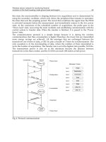
the probe . . . . . . . . . . . . . . . . . . . . . . . . . . . . . . . .
2.4 Types of Face Change during a face walk . . . . . . . . . . . . . .
2.5 Cell-based forwarding results in the solid path and positionbased Greedy forwarding in the dotted path . . . . . . . . . . . .
2.6 Planarization effected by two trees . . . . . . . . . . . . . . . . .
√
2.7 Crossing edge in a QUDG with R/r <= 2 . . . . . . . . . . . . . .
2.8 Any 1-local routing algorithm is defeated by G1/G2 if all routing
functions are derangements. . . . . . . . . . . . . . . . . . . . . .
2.9 The four possible combinations of derangements for local routing
functions fa′ and fe′ . . . . . . . . . . . . . . . . . . . . . . . . . . .
2.10 Virtual grid formed from dual graphs to border the void (taken
from [9]) . . . . . . . . . . . . . . . . . . . . . . . . . . . . . . . . .
2.11 Example of greedy-hull-greedy (GHG) routing (taken from [31])
3.1
3.2
3.3
3.4
3.5

.
.

2

8
9

. 11
. 12
. 17
. 18
. 22
. 24
. 24
. 26
. 28

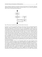
Overview of GDSTR tree traversal. . . . . . . . . . . . . . . . . . . .
Illustration of routing using GDSTR-3D . . . . . . . . . . . . . . .
Illustration of how undeliverable packet is handled in GDSTR-3D
Different 3D hull alternatives . . . . . . . . . . . . . . . . . . . . .
Handshake between neighbour nodes for limiting number of children . . . . . . . . . . . . . . . . . . . . . . . . . . . . . . . . . . . .

33
37
38
41
45

4.1 Classification of message exchanged among nodes for GDSTR . . 49
4.2 Functional diagram of GDSTR implementation . . . . . . . . . . . 53

iv

5.1 Comparison of success rates for GDSTR-3D, CLDP+GFR, GDSTR
for 3D networks. . . . . . . . . . . . . . . . . . . . . . . . . . . . . . 57
5.2 Plot of routing stretch of GDSTR-3D and GDSTR [25] 2-hop with
fragmentation against network density for 3D networks . . . . . . 59
5.3 Plot of routing stretch of CLDP+GFR [15] against network density
for 3D networks . . . . . . . . . . . . . . . . . . . . . . . . . . . . . 59
5.4 Plot of hop stretch against network size for GDSTR, GDSTR-3D
in low density . . . . . . . . . . . . . . . . . . . . . . . . . . . . . . . 60
5.5 Plot of hop stretch against network size for GDSTR, GDSTR-3D
in high density . . . . . . . . . . . . . . . . . . . . . . . . . . . . . . 60
5.6 Plot of hop stretch against network size for CLDP+GFR . . . . . . 61
5.7 Comparison of average storage requirements per Node for GDSTR,
GDSTR-3D and CLDP+GFR . . . . . . . . . . . . . . . . . . . . . . 62
5.8 Comparison of maximum storage requirements per Node for GDSTR,
GDSTR-3D and CLDP+GFR . . . . . . . . . . . . . . . . . . . . . . 63
5.9 Average storage for GDSTR, GDSTR-3D and CLDP+GFR in low
density . . . . . . . . . . . . . . . . . . . . . . . . . . . . . . . . . . . 63
5.10 Average storage for GDSTR, GDSTR-3D and CLDP+GFR in high
density against different network size . . . . . . . . . . . . . . . . . 64
5.11 Maximum storage for GDSTR, GDSTR-3D and CLDP+GFR in low
density . . . . . . . . . . . . . . . . . . . . . . . . . . . . . . . . . . . 64
5.12 Maximum storage for GDSTR, GDSTR-3D and CLDP+GFR in high
density against different network size . . . . . . . . . . . . . . . . . 65
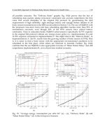
5.13 Plot of beacon message overhead required to converge per node
against network density for GDSTR, GDSTR-3D . . . . . . . . . . 67
5.14 Plot of beacon message overhead required to converge per node
against network density for CLDP+GFR . . . . . . . . . . . . . . . 67
5.15 Plot of beacon message overhead required to converge per node

against network density for GDSTR, GDSTR-3D in 2-hop with
fragmentation . . . . . . . . . . . . . . . . . . . . . . . . . . . . . . 68
5.16 Plot of beacon message overhead required to converge per node
against network density for CLDP+GFR . . . . . . . . . . . . . . . 68
5.17 Plot of total transmission overhead required to converge per node
against network size for GDSTR, GDSTR-3D in low density . . . . 69
5.18 Plot of total transmission overhead required to converge per node
against network size for GDSTR, GDSTR-3D in high density . . . 69
5.19 Plot of total transmission overhead required to converge per node
against network size for CLDP+GFR . . . . . . . . . . . . . . . . . . 70

v


5.20 Topology divided into routing regions w.r.t node’s hop count to
the roots . . . . . . . . . . . . . . . . . . . . . . . . . . . . . . . . .
5.21 Example of how direction of routing affect hop stretch . . . . . .
5.22 Examples of poor and good selection of center for spheres . . . .
5.23 Example of false positives created by projection of 3D convex hull
on 2D . . . . . . . . . . . . . . . . . . . . . . . . . . . . . . . . . .
5.24 Void regions are located to one side of the topology . . . . . . . .
5.25 False positives caused by overlapping regions in the network . .
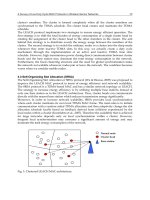
5.26 Nodes sending data to base station . . . . . . . . . . . . . . . . .
5.27 Failure of best intersection and first intersection face routing . .
5.28 Failure of closest node and closest point face routing . . . . . . .

vi

. 71
. 73

. 73
.
.
.
.
.
.

74
76
76
77
78
79


Abstract
Wireless sensor networks have been deployed in various applications like
habitat or environment monitoring and the network is likely to grow in size.
Compared to traditional ad-hoc routing, geographic routing algorithms are
attractive for such networks. Many existing works on geographic routing are
done for two dimensional topologies. But in real world, many sensor networks are deployed in three dimensions. Greedy Distributed Spanning Tree
Routing (GDSTR) [25] have shown to perform better than some well-known algorithms like CLDP+GFR [15] for 2D networks. In this work, we implemented
GDSTR in TinyOS, developed a 3D extension of the algorithm, called GDSTR3D, and compared the performance of the new algorithm to GDSTR [25] and
CLDP+GFR [15]. Our evaluations showed that GDSTR-3D performs better
than 2D algorithms with comparable or even lower cost. Our GDSTR-3D using spheres performs 25% better than GDSTR-2D and 85% better than CLDP
in terms of hop stretch.

vii

Chapter 1
Introduction
1.1 Background
Geographic routing or position-based routing is a routing approach that uses
the location information of the nodes in the network. The idea of using location information for routing dates back to the 1980’s in the area of packet
radio networks [39] and interconnection networks [8]. Unlike topology-based
routing, geographic routing relies mainly on location information instead of
topological connectivity to make forwarding decisions. Their storage requirement depends mostly on network density rather than network size and hence
provides scalability. In geographic routing, each node must know its location,
the location of its neighbours and that of the packet destination.
The basic technique in geographic routing is called greedy forwarding,
where packets are routed to a neighbouring node that is geographically closer
to the destination than itself in every hop. Even though greedy forwarding
is efficient, it will fail in cases where a node is unable to find a neighbour
geographically closer to the destination than itself. This occurrence is called
a communication void. This can be seen in the Figure 1.1 where node S needs
to send a packet to the destination node (D) and there is no neighbour closer

1


Figure 1.1: Example of communication void

to D than S. The node S is called a local minimum. In such case, an alternate approach is needed to handle this void. Prior research have focused on
developing an efficient algorithm to handle situations when greedy forwarding fails [12, 15, 26]. Since geographic routing relies on position information,
another associated research problem is to determine the location of nodes
in terms of either physical coordinates that reflect actual node positions or
virtual coordinates [34, 27].
Void-handling techniques are used to route around void and once the

packet encounters a node whose distance is less than the local minimum,
greedy forwarding will be resumed. While flooding is simple and effective in
packet delivery, it is inefficient in terms of resource utilization. Hence, the
following are some desirable properties when choosing a void-handling technique:
• Void-handling should involve as few nodes as possible. It is preferable to
handle it at the local minimum itself.
• It is preferable that unless there is data traffic at the local minimum, it
should not incur any overhead in the idle period.
• Greedy forwarding exploits location information. Hence, it is desirable to
2


have the void-handling use this information rather than any additional
information.
• The path obtained from the technique should hopefully be comparable
to the optimal path attainable in the given topology.
• The void-handling technique should be resource-efficient.
Our algorithm was implemented on Wireless Sensor Network (WSN) in
TinyOS, an open source operating system for WSN. We would like to give
an overview about the platform. There is growing interest in using sensors in
real-life applications like habitat monitoring, traffic monitoring and they are
likely to be deployed in large numbers. Hence, any routing algorithm for sensor networks should be scalable. The memory available on sensors are small.
For example, a TelosB mote only has 10KB RAM and 1MB flash [2]. Under
laboratory conditions, wireless sensors are powered by batteries or USB [2].
But field deployments might need to be battery-powered. Battery-powered
sensors have energy constraints.
The source code of TinyOS is in nesC which does not provide dynamic
memory allocation [4]. We can achieve dynamic memory allocation by creating a shared memory pool and dynamically allocating memory from it [28]
which means that the call-graph is fully known at compile-time [4]. Hence
a good routing algorithm for WSN needs to consider both storage and energy

constraints.

1.2 Motivation
While there has been much work on geographic routing, prior work mostly
deal with routing on Euclidean 2D topologies. Many 2D void-handling techniques proposed are based on planarization and face walking. Some algo3


rithms maintain routing information in formats like tables, cells or trees to
handle voids. Another approach is a beacon-based one where the algorithm
assigns landmarks across the network which help a packet to navigate out of
the void region. All these algorithms address routing on 2D topology. But,
there are some real world scenarios, like networks within a building, that
demand three-dimensional routing.
Even though greedy forwarding works in 3D topologies, it can also encounter communication voids. On 3D geographic routing, Durocher et al. [3]
showed that there is no deterministic local routing algorithm for 3D networks that guarantees the delivery of messages on any arbitrary 3D topology.
In their proof, they showed that any deterministic 1-local routing algorithm
which can exist will have a graph G for which it is defeated and extend the
proof to any k-local algorithm. Hence, there is no local memoryless algorithm
which can guarantee delivery on any arbitrarily connected 3D network. Flury
et al. [9] and Liu et al. [31] have attempted to address the problem of 3D geographic routing. While their work extend the ideas of 2D algorithm to 3D,
their results are not encouraging in terms of performance and simplicity of
solution.
In this light, we explore the trade-off between performance and cost for
geographic routing algorithms in 3D networks in this dissertation.

1.3 Research Contributions
There are two main contributions in the thesis: first, we implemented GDSTR [25]
in nesC on the TinyOS platform for wireless sensor networks; second, GDSTR
was further extended to 3D and evaluated on 3D topologies against two wellknown 2D geographic routing algorithms, GDSTR [25] and CLDP+GFR [15].
GDSTR maintains minimal-path spanning tree and each node in the tree

4


maintains a 2D convex hull enclosing the locations of all the nodes in the
subtree rooted at this node. We implement GDSTR on TinyOS and extended it
for 3D networks by replacing the 2D convex hull with 3D geometric structures
like 3D convex hull and sphere. The storage required by GDSTR is proportional to the average number of children per node. Storage affects the amount
of information to be exchanged between nodes (message overhead) which in
turn impact the energy consumed. Wireless sensors have small memory. So,
we bound the storage requirement of GDSTR by limiting the maximum number of children a node can have for a tree.
Our evaluation shows that GDSTR-3D (with spheres) performs better than
the 2D algorithms under most scenarios.

1.4 Organization
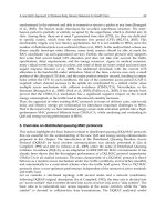
The rest of this dissertation is organized as follows: Chapter 2 provides a
literature review of existing research relevant to our work. Chapter 3 describes
our GDSTR-3D routing algorithm. Chapter 4 describes the implementation
of our algorithm in TinyOS. Finally, Chapter 5 describes our experimental
results and evaluation and Chapter 6 concludes our discussion.

5


Chapter 2
Related Work
One of the primary research problems in geographic routing is void-handling.
In this section, we provide a survey of the existing work related to our work.
We classify the literature based on their approach to solve the problem. Broadly,
it can be classified as solutions for 2D and 3D networks. The basic assumption in all of these algorithms is that each node knows its location and the

location of its neighbours and packet destination. There might be other assumptions on the underlying topology such as the dimension of topology,
symmetry of links, radio range, etc.

2.1 2D Planar-graph Based
This is the most widely used void-handling technique that makes use of properties of a planar graph. From graph theory, a planar graph is defined as a
graph that can be embedded in a plane without any intersecting edges. The
right hand rule is used for traversing a planar graph to find a path between
given source and destination. The right hand rule states that, by keeping one’s
right hand against the wall while moving forward, one is likely to traverse every wall in a maze. The intuition behind such approach is that a packet will

6


be able to exit the void region by performing a face walk starting from the local
minimum. Ideally, due to a wireless node’s circular radio range the resulting
topology should obey unit disk graph (UDG)) assumption. According to this
assumption, two nodes are connected if the distance between them is less
than the common radio range of the nodes. But in real world, the underlying
topology does not obey this rule and hence the topology is not always planar.
The network has to be planarized for the routing algorithm to work.
A complete planar-based protocol should have a planarization algorithm
and a planar-graph traversal algorithm for routing. Complete planar-based
void-handling techniques include Greedy Perimeter Stateless Routing (GPSR) [12],
by-pass routing in Priority-based Stateless Geo-Routing (PSGR) [6] and RequestResponse (RR) in Beacon-less routing (BLR) [5]. We will briefly discuss planarization algorithms and face routing, which is a planar-graph traversal
algorithm. Then, we will summarize some planar-graph based solutions in
existing research.

2.1.1 Planarization
Existing works on planarization algorithms include RNG (Relative Neighbourhood Graphs), GG (Gabriel Graphs) [12]. The concept behind both GG and
RNG is the same. They try to planarize a given graph by removing a link if

there exists a node (witness) in a bounded area around the link. The only
difference lies in the definition of the bounded area as can be seen in Figure
2.1. These algorithms assume that the given topology obeys UDG assumption.
Real world topologies does not obey UDG rule [15].
Hence in a non-UDG case, Kim et al. [16] have shown that removal of a
link may cause the following pathologies:
• Network partitioning: There could be critical links which connects two
7


Figure 2.1: Planarization by GG, RNG and occurrence of pathology in a nonUDG case

sub graphs and removing such a link might disconnect the network.
• Asymmetric links: Sometimes the witness node is visible to only one
end of the link. This will cause the node which can see the witness to
remove the link making it asymmetric. It will be problematic as most of
the existing routing algorithm assume symmetric links.
• Crossing links: Crossing links occur due to either obstacles or localization errors, when there is a node within the bounded area not visible to
both ends of the link. Both RNG and GG cannot detect such crossing
links. This can cause routing failures as shown in the Figure 2.2 where
node S sends a packet to node D. S sends the packet to the neighbour
closer to D which becomes the local minimum. Even after walking the
entire face, the local minimum cannot find a next hop and routing fails.
A solution was proposed for the pathologies called the Mutual Witness
(MW)[ [15], [36]]. A node will remove a link only if there exists a witness
seen by both ends of the link in the given bounded area. This can be verified
by a handshake sending the list of its visible neighbours and looking for mutually visible neighbour to the other end in the bounded area. This fix resolves
8

Figure 2.2: Routing failure due to crossing links by obstacles

only the first two pathologies but it still cannot remove crossing links. Kim et
al. [15] in his work called Cross-Link Detection Protocol (CLDP) provides a solution to this problem by removing such crossing links. CLDP will be discussed
later in the literature.

CLDP
Kim et al. [15] have identified that existing planarization algorithms like RNG
and GG does not remove cross-links and fail to planarize the graph when UDG
assumption is violated. The Mutual Witness (MW) fix also does not remove
crossing links due to the same UDG assumption. Hence a protocol called
Cross-Link Detection Protocol (CLDP) [15] was proposed by them.
In CLDP, each node in an entirely distributed fashion probes each of its
links to see if it is crossed (by geographic location) by any other links. A probe
traverses the graph by right hand rule and initially contains the location of the
end points of the link being probed. When the probe encounters a crossing,
it records the fact in the probe message so that when it reaches back to the

9


sender, the sender can remove either of the crossed links after a series of
message exchanges. The sender removes the agreed link by marking it nonroutable. The next probe will traverse the modified topology.
When a link is added to the underlying graph, CLDP awakens the adjacent
dormant links causing the links on the corresponding face to be probed again.
When a link is deleted from the network, then probing adjacent links might restore some links marked as non-routable by previous probes. However, CLDP
does not always remove cross-links. When a probe traverses a link in both
directions (highlighted in Figure 2.3), it means that the link is a critical link
i.e removing such a link would partition the graph. Hence,it does not remove
such cross-links. Note that the subgraph produced by CLDP is used only by

the face routing part and greedy forwarding uses the entire graph. In their
work, Kim et al. [15], GPSR [12] is run on the routable subgraph produced by
CLDP. However, CLDP can run with any face traversal algorithm. CLDP+GFR
(CLDP with GPSR) was evaluated on TOSSIM, a TinyOS simulator for wireless sensors and on real motes. Results have shown that the performance of
CLDP+GFR [15] is better than the original GPSR [12]. They have also proved
that CLDP prevents routing failures in an arbitrary connected graph [16].

Lazy CLDP
The probing of links from each node causes high message overhead in CLDP.
Hence, Lazy Cross-link Removal (LCR) by Kim et al. [17], removes cross-links
lazily only when geographic routing fails. Their argument is that the class
of cross-links which causes routing failures are narrower (only during void)
and it is sufficient to remove links causing face walk loops to ensure delivery. This means that in addition to critical links, LCR also keeps cross-links
that do not cause routing failures. LCR doesn’t efficiently support routing
to arbitrary locations. LCR uses face walk loops to detect cross-links and so
10


Figure 2.3: Identifying critical links removing which will partition the network.
As shown, critical links are traversed in both directions by the probe

cannot distinguish between cross-links and unreachable destination. Hence,
any-any routing in LCR can only be done using a location service to detect
unreachable address. Handling link failures are similar to that of CLDP i.e.
It awakens all the links in the failed planar subgraph and do CLDP probing again. LCR also removes looped walk without cross-links by recursively
searching adjacent faces for cross-links. Their experimental results both on
simulation and real networks have shown that it does incur much less overhead than CLDP. Depending on which link is probed first, the same network
can produce different subgraphs in CLDP.

2.1.2 Face routing

Face routing is a typical planar graph traversal technique which involves
walking adjacent faces using right hand rule towards destination (D). These
algorithms are classified as follows based on where a walk exits a face to the
next face (please refer Figure 2.4):
• Best Intersection (Compass [18], AFR [20]): After a face is entirely
toured using right hand rule, face change occurs at the link closest to D
11


Figure 2.4: Types of Face Change during a face walk

that intersect the line SD on the current face.
• First Intersection (GPSR [12], GFG [1]): Face change occurs at the first
intersection of the link as seen by the face walk with the line SD at a
node closer to D than local minimum.
• Closest Node (GOAFR+ [19]): After walking the entire face, face change
occurs at the node closest to the destination (D) on that face.
• Closest Point (GOAFR, [21]): After walking the entire face, face change
occurs at the closest point to D in the face.
However, face walking may not be an effective solution in real world networks. Kim et al. [16] have shown ways in which some existing planarization
techniques fail with realistic, non-ideal radios. They have found that ’first intersection’ and ’closest node’ don’t always work and they have also provided
topologies in which these face walks fail to find the next hop.

12


BLR
Request-Response (RR) is a technique used in BLR [5]. In RR, a complete
planar subgraph is not constructed before hand. It will planarize the graph
around the void region only when it encounters one during routing. A void

node broadcasts a request and all neighbours reply with a message having
their positions. Then the void node constructs a planar subgraph around the
area using Gabriel Graph (GG) algorithm and forwards the packet to the next
node using right hand rule. Due to on-demand planarization, this approach
increases the packet delivery latency.

PSGR
In Priority-based Stateless Geo-Routing (PSGR) [6], a void node moves the
packet to a by-pass node without exploiting prior-knowledge of network topology. A void node performs a sweeping rule (left/right-hand rule) by scanning
its neighbourhood in chosen direction (clockwise/counter-clockwise) on the
fly. If it is able to find a neighbour node within 180◦ , it forwards the packet
to that node and subsequent forwarding happens in the same chosen direction. Otherwise, the node will repeat the same in the other direction and forward the packet to the first neighbour node in that direction. The by-passing
will also change traversal direction when the packet crosses the line passing
through the source (S) and destination (D). This algorithm will only work if
the underlying graph is planar.

GPSR
Perimeter routing proposed by Greedy Perimeter Stateless Routing (GPSR) [12]
is a complete void-handling solution that consists of distributed planarization
algorithm using either RNG or GG and a graph traversal algorithm. All nodes

13


run the distributed planarization algorithm periodically so that a planar subgraph of the original network is always maintained. When a packet encounters void, it switches to face traversal algorithm. The void node information is
recorded into the packet and face walking is done by first intersection. When
it reaches a node closer to the destination than the local minimum, the algorithm switches back to greedy forwarding. The void node information on the
packet ensure that the next greedy forwarding is resumed at the node closer
to the destination than itself thereby preventing routing loops. This technique
is based on UDG assumption and hence suffers routing failures in a non-UDG

case [15].

GOAFR
Kuhn et al. performs other face routing (OFR) based on closest point face routing in the proposed algorithm Greedy Other Adaptive Face Routing (GOAFR) [21].
Planarization is done by GG. The idea in GOAFR is to find the optimal path
in a worst-case scenario. i.e. when one side of the face extends infinitely long
and if the face walk chooses this side, then the cost of stretch and routing time
will be considerably high. GOAFR aims to bound this routing time. According to GOAFR, a void node performs OFR along one direction say clockwise
within radius of one hop. If that fails, the node switches to the other direction
(counter-clockwise) and performs OFR within one-hop radius. If both fails,
then it extends its radius to the next increment and repeats the same until a
routing decision can be made. GOAFR has the same disadvantage as GPSR
because of UDG assumption.

14


2.2 2D topology-based
Topology-based void-handling makes use of connectivity information to route
around the void. The simplest solution when a void occurs is flooding. But
network wide flooding can be expensive in terms resource utilization. Hence,
some topology based algorithms attempt controlled flooding or partial flooding.
Topology-based techniques can be classified into two namely proactive and
reactive protocols. Proactive algorithms are those which precompute routing
structures to handle void. Reactive algorithms handle void on-demand and is
categorized into two depending on data flow i.e whether the packet is a onetime message or packets to the same destination are sent often. In the former
case, flooding can be used to reach the destination and in the latter, route will
be discovered from the void node and the routing information is maintained
in a table.

2.2.1 Reactive protocols
Reactive protocols handle voids only during routing when a packet gets stuck
in a void. Some solutions perform limited flooding as in Cartesian Routing [8]
and one-hop flooding [37]. In Geographic Routing Algorithm (GRA) [38], when
a packet encounters void node, the node performs on-demand route discovery by breadth first search. The discovered route is updated in a routing
table and the stuck packet is routed to the destination by partial hop by hop
routing (PHR). Partial Source Routing (PSR) is an on-demand stateless voidhandling technique. It consists of two phases, (a) the partial path discovery
phase where a void node performs expanded ring search for route discovery
and (b) the source packet forwarding phase where the void node uses already
discovered route in its routing table to do source routing.
15


2.2.2 Pro-active protocols
As the name suggests, proactive protocols try to be prepared for voids before
a packet encounters one. In this section, we describe two such protocols:
Robotic Routing Protocol (RRP) and Greedy Distributed Spanning Tree Routing (GDSTR).

RRP
Robotic Routing Protocol (RRP) [13] is a Grid based recovery technique. In a
two dimensional network the surface is logically partitioned into cells/grids
√
with edge length dG ≤ dR / 2 where dR is the transmission radius. In other
words, all nodes in a cell are one-hop neighbours and can communicate directly. Each node in the network maintains the routing information about its
neighbor cells as well as its one-hop neighbour nodes. The node knows which
neighbour cells are empty or occupied and how to reach the occupied neighbour cells by associating them with neighbour nodes. A packet is forwarded
by cell-cell greedy forwarding rather than the usual node-node. When void
occurs, the grid structure is used to approximate the shape of the obstacles
by walking over cells (refer Figure 2.5) around the void region until greedy
forwarding can be resumed. Simple Right hand rule is performed between the

cells to walk around the obstacle/empty cell.

GDSTR
Greedy Distributed Spanning Tree Routing (GDSTR) by Leong et al. [25] uses
minimal path spanning trees called hull trees for void-handling. A hull tree is
a spanning tree where each node has an associated convex hull enclosing the
locations of all the nodes in the subtree rooted at this node. Two trees rooted
at extreme ends of the network are precomputed. Each node stores its own

16


Figure 2.5: Cell-based forwarding results in the solid path and position-based
Greedy forwarding in the dotted path

convex hull and that of its children for each tree. When a packet is stuck,
the void node chooses the tree whose root is closer to the destination as the
routing tree. It checks if the destination is contained in the convex hull of any
of its child nodes. If it is contained, then the node forwards the packet to that
child whose convex hull contains the destination node. If the destination is
not contained in any of the convex hulls, then it will forward the packet to its
parent. The process is repeated until a routing decision can be made, i.e (1)
the destination node is reached or (2) a node where greedy forwarding can be
resumed is reached in which case greedy forwarding will be resumed or (3)
the destination is marked as unreachable.
Two trees rooted at the extreme ends are used to effectively approximate
a planarization as illustrated in the Figure 2.6. GDSTR performs better in
sparse networks with large voids than face routing algorithms as it uses global
information using precomputed hull trees unlike the face routing algorithms.
However when the voids are small, face routing algorithm achieves slightly a

17