THE FREQUENCY DOMAIN
Bạn đang xem bản rút gọn của tài liệu. Xem và tải ngay bản đầy đủ của tài liệu tại đây (581.48 KB, 14 trang )
9. THE FREQUENCY DOMAIN
9.1 Introduction
Much signal processing is done in a mathematical space known as the frequency domain.
In order to represent data in the frequency domain, some transform is necessary. The most
studied one is the Fourier transform.
In 1807, Jean Baptiste Joseph Fourier presented the results of his study of heat propagation
and diffusion to the Institut de France. In his presentation, he claimed that any periodic
signal could be represented by a series of sinusoids. Though this concept was initially met
with resistance, it has since been used in numerous developments in mathematics, science,
and engineering. This concept is the basis for what we know today as the Fourier series.
Figure 9.1 shows how a square wave can be created by a composition of sinusoids. These
sinusoids vary in frequency and amplitude.
Figure 9.1 (a) Fundamental frequency: sine(x); (b) Fundamental plus 16 harmonics:
sine(x) + sine(3x)/3 + sine(5x)/5...
What this means to us is that any signal is composed of different frequencies. This applies
to 1-dimensional signals such as an audio signal going to a speaker or a 2-dimensional
signal such as an image.
A prism is a commonly used device to demonstrate how a signal is a composition of
signals of varying frequencies. As white light passes through a prism, the prism breaks the
light into its component frequencies revealing a full color spectrum.
The spatial frequency of an image refers to the rate at which the pixel intensities change.
Figure 9.2 shows an image consisting of different frequencies. The high frequencies are
concentrated around the axes dividing the image into quadrants. High frequencies are
noted by concentrations of large amplitude swings in the small checkerboard pattern. The
corners have lower frequencies. Low spatial frequencies are noted by large areas of nearly
constant values.
Figure 9.2 Image of varying frequencies
The easiest way to determine the frequency composition of signals is to inspect that signal
in the frequency domain. The frequency domain shows the magnitude of different
frequency components. A simple example of a Fourier transform is a cosine wave. Figure
9.3 shows a simple 1-dimensional cosine wave and its Fourier transform. Since there is
only one sinusoidal component in the cosine wave, one component is displayed in the
frequency domain. You will notice that the frequency domain represents data as both
positive and negative frequencies.
Many different transforms are used in image processing (far too many begin with the letter
H: Hilbert, Hartley, Hough, Hotelling, Hadamard, and Haar). Due to its wide range of
applications in image processing, the Fourier transform is one of the most popular (Figure
9.5). It operates on a continuous function of infinite length. The Fourier transform of a 2dimensional function is shown mathematically as
H ( u, v ) =
∞ ∞
∫ ∫ h ( x, y ) e
− j 2π ( ux + vy )
dxdy
− ∞− ∞
where
j = −1
and
e ± jx = cos( x ) ± j sin( x)
it is also possible to transform image data from the frequency domain back to the spatial
domain. This is done with an inverse Fourier transform:
h ( x, y ) =
∞ ∞
∫ ∫ H (u, v)e
− j 2π ( ux + vy )
dudv
− ∞− ∞
Figure 9.3 Cosine wave and its Fourier transform
It quickly becomes evident that the two operations are very similar with a minus sign in
the exponent being the only difference. Of course, the functions being operated on are
different, one being a spatial function, the other being a function of frequency. There is
also a corresponding change in variables.
Figure 9.4 Fourier Transform of a spot: (a) original image; (b) Fourier Transform.
(This picture is taken from Figure 7.5, Chapter 7, [2]).
In the frequency domain, u represents the spatial frequency along the original image's x
axis and v represents the spatial frequency along the y axis. In the center of the image u
and v have their origin.
The Fourier transform deals with complex numbers (Figure 9.6). It is not immediately
obvious what the real and imaginary parts represent. Another way to represent the data is
with its sign and magnitude. The magnitude is expressed as
H (u , v) = R 2 (u , v) + I 2 (u, v)
and phase as
I (u , v )
θ (u , v) + tan −1
R (u , v)
where R(u,v) is the real part and I(u,v) is the imaginary. The magnitude is the amplitude of
sine and cosine waves in the Fourier transform formula. As expected, 0 is the phase of the
sine and cosine waves. This information along with the frequency, allows us to fully
specify the sine and cosine components of an image. Remember that the frequency is
dependent on the pixel location in the transform. The further from the origin it is, the
higher the spatial frequency it represents.
magnitude
θ
Real
Figure 9.5 Relationship between imaginary number and phase and magnitude.
9.2 Discrete Fourier Transform
When working with digital images, we are never given a continuous function, we must
work with a finite number of discrete samples. These samples are the pixels that compose
an image. Computer analysis of images requires the discrete Fourier transform.
The discrete Fourier transform is a special case of the continuous Fourier transform.
Figure 9.7 shows how data for the Fourier transform and the discrete Fourier transform
differ. In Figure 9.7(a), the continuous function can serve as valid input into the Fourier
transform. In Figure 9.7(b), the data is sampled. There is still an infinite number of data
points. In Figure 9.7(c), the data is truncated to capture a finite number of samples on
which to operate. Both the sampling and truncating process cause problems in the
transformation if not treated properly.
The formula to compute the discrete Fourier transform on an M x N size image is
H(u, v) =
1
MN
M −1 N −1
∑∑ h(x, y)e
− j2 22 22+ vy/N)
x =0 y =0
The formula to return to the spatial domain is
h ( x, y ) =
M −1 N −1
∑∑ H (u, v)e
j 2π ( ux / M + vy / N )
x =0 y =0
Again it can be seen that the operations for the DFT and inverse DFT are very similar. In
fact, the code to perform these operations can be the same taking note of the direction of
the transform and setting the sign of the exponent accordingly.
There are problems associated with data sampling and truncation. Truncating a data set to
a finite number of samples creates a ringing known as Gibb's phenomenon. This ringing
distorts the spectral information in the frequency domain. The width of the ringing can be
reduced by increasing the number of data samples. This will not reduce the amplitude of
the ringing. This ringing can be seen in either domain. Truncating data in the spatial
domain causes ringing in the frequency domain. Truncating data in the frequency domain
causes ringing in the spatial domain.
Figure 9.6 (a) Continuous function; (b) sampled; (c) sampled and truncated
The discrete Fourier transform expects the input data to be periodic, and the first sample is
expected to follow the last sample. The amplitude of the ringing is a function of the
difference between the amplitude of the first and last samples. To reduce this
discontinuity, we can multiply the data by a windowing function (sometimes called
window weighting functions) before the Fourier transform is performed.
There are a number of window functions, each with its set of advantages and
disadvantages. Figure 9.8 shows some popular window functions. N is the number of
samples in the data set. The Bartlett window is the simplest to compute requiring no sine
or cosine computations. Ideally the data in the middle of the sample set is attenuated very
little by the window function.
The equation for the Bartlett window is
2n
N − 1
w(n) =
2 − 2 n
N −1
0≤n<
N −1
2
N −1
≤ n ≤ N −1
2
The equation for the Hamming window is
w(n) =
1
2πn
1 − cos
2
N − 1
The equation for the Hamming window is
2πn
w(n) = 0.54 − 0.46 cos
N −1
The equation for a Blackman window is
2πn
4πn
w(n) = 0.42 − 0.5 cos
+ 0.08 cos
N −1
N −1
Figure 9.7 1-dimensional window function
Just like many other functions, 1-dimensional windows can be converted into 2dimensional windows by the following equation
(
f ( x, y ) = w x 2 + y 2
)
that the original data be periodic. There are some great discontinuities at the truncation
edges. Window functions attenuate all values at the truncation edges. These great
discontinuities are hence removed. Figure 9.8 also shows the truncated function after
windowing.
Figure 9.8 Truncated function, what DFT thinks, results of window operation.
Window functions attenuate the original image data. Window selection requires a
compromise between how much you can afford to attenuate image data and how much
spectral degradation you can tolerate.
9.3 Fast Fourier Transform
The discrete Fourier transform is computationally intensive requiring N2 complex
multiplications for a set of N elements. This problem is exacerbated when working with 2dimensional data like images. An image of size M x M will require (M2)2 or M4 complex
multiplications.
Fortunately, in 1942, it was discovered that the discrete Fourier transform of length N
could be rewritten as the sum of two Fourier transforms of length N/2. This concept can be
recursively applied to the data set until it is reduced to transforms of only two points. Due
partially to the lack of computing power, it wasn't until the mid 1960s that this discovery
was put into practical application. In 1965, JW. Cooley and J.W. Tukey applied this
finding at Bell Labs to filter noisy signals.
This divide and conquer technique is known as the fast Fourier transform. It reduces the
number of complex multiplications from N2 to the order of Nlog2N. Table 7.1 shows the
computations and time required to perform the DFT directly and via the FFT. It is
assumed that each complex multiply takes 1 microsecond.
This savings is substantial especially when image processing. The FFT is separable, which
makes Fourier transforms even easier to do. Because of the separability, we can reduce the
FFT operation from a 2-dimensional operation to two 1-dimensional operations. First we
compute the FFT of the rows of an image and then follow up with the FFT of the columns.
For an image of size M x N, this requires N + M FFTs to be computed. The order of
NMlog2NM computations are required to transform our image. Table 7.2 shows the
computations and time required to perform the DFT directly and via the FFT.
There are some considerations to keep in mind when transforming data to the frequency
domain via the FFT. First, since the FFT algorithm recursively divides the data down, the
dimensions of the image must be powers of 2 (N = 2j and M = 2k where j and k can be any
number). Chances are pretty good that your image dimensions are not a power of 2. Your
image data set can be expanded to the next legal size by surrounding the image with zeros.
This is called zero-padding. You could also scale the image up to the next legal size or cut
the image down at the next valid size. For algorithms that remove this power of 2
restriction, see the last section of this chapter.
Table 7.1 Savings when using the FFT on 1-dimensional data
Size of data DFT
set
multiplication
1E6
1024
DFT time
FFT Time
1 sec
FFT
multiplication
10,240
0.01 sec
8192
67E6
67 sec
106,496
0.1 sec
65536
4E9
71 min
1,048,576
1.0 sec
1048576
1E12
305 hr
20.971.520
20.9 sec
Table 7.2 Savings when using the FFT on 2-dimensional data
Image size
256*256
512*512
1024*1024
2048*2048
DFT
multiplication
4.3E 9
6.8E10
1.1E12
1.8 E 13
DFT
time
71 min
19 hr
12 days
203
days
FFT
multiplication
1,048,576
4,718,592
20,971,520
92,274,688
FFT Time
1.0 sec
4.8 sec
21.0 sec
92.2 sec
The 1-dimentional FFT function can be broken down into two main functions. The first is
the scrambling routine. Proper reordering of the data can take advantage of the periodicity
and symmetry of recursive DFT computation. The scrambling routine is very simple. A bit
reversed index is computed for each element in the data array. The data is then swapped
with the data pointed to by the bit-reversed index. For example, suppose you are
computing the FFT for an 8 element array. The data element at address 1 (001) will be
swapped with the data at address 4 (100). Not all data is swapped since some indices are
bit-reversals of themselves (000, 010, 101, and 111) (Figure 9.10).
000
data 0
data 0
001
data 1
data 4
010
data 2
data 2
011
data 3
data 6
100
data 4
data 1
101
data 5
data 5
110
data 6
data 3
111
data 7
data 0
Figure 9.9 Bit-reversal operation
The second part of the FFT function is the butterflies function. The butterflies function
divides the set of data points down and performs a series of two point discrete Fourier
transforms. The function is named after the flow graph that represents the basic operation
of each stage: one multiplication and two additions (Figure 9.10).
Figure 9.10 Basic butterfly flow graph.
Remember that the FFT is not a different transform than the DFT, but a family of more
efficient algorithms to accomplish the data transform. Usually when one speeds up an
algorithm, this speed up comes at a cost. With the FFT, the cost is complexity. There is
complexity in the bookkeeping and algorithm execution. The computational savings,
however, do not come at the expense of accuracy.
Now that you can generate image frequency data, it's time to display it. There are some
difficulties to overcome when displaying the frequency spectrum of an image. The first
arises because of the wide dynamic range of the data resulting from the discrete Fourier
transform. Each data point is represented as a floating point number and is no longer
limited to values from 0 to 255. This data must be scaled back down to put in a displayable
format. A simple linear quantization does not always yield the best results, as many times
the low amplitude data points get lost. The zero frequency term is usually the largest
single component. It is also the least interesting point when inspecting the image spectrum.
A common solution to this problem is to display the logarithm of the spectrum rather than
the spectrum itself. The display function is
D(u , v) = x log[1 + H (u , v) ]
where c is a scaling constant and H(u,v) is the magnitude of the frequency data to display.
The addition of 1 insures that the pixel value 0 does not get passed to the logarithm
function.
Sometimes the logarithm function alone is not enough to display the range of interest. If
there is high contrast in the output spectrum using only the logarithm function, you can
clamp the extreme values. The rest of the data can be scaled appropriately using the
logarithm function above.
Since scientists and engineers were brought up using the Cartesian coordinate system, they
like image spectra displayed that way. An unaltered image spectrum will have the zero
component displayed in the upper left hand corner of the image corresponding to pixel
zero. The conventional way of displaying image spectra is by shifting the image both
horizontally and vertically by half the image width and height. Figure 9.11 shows the
image spectrum before and after this shifting. All spectra shown thus far have been
displayed in this conventional way. This format is referred to as ordered (as opposed to
unordered).
Now that we can view the image frequency data, how do we interpret it? Each pixel in the
spectrum represents a change in the spatial frequency of one cycle per image width. The
origin (at the center of the ordered image) is the constant term, sometimes referred to as
the DC term (from electrical engineering's direct current). If every pixel in the image were
gray, there would only be one value in the frequency spectrum. It would be at the origin.
The next pixel to the right of the origin represents 1 cycle per image width. The next pixel
to the right represents 2 cycles per image width and so forth. The further from the origin a
pixel value is, the higher the spatial frequency it represents. You will notice that typically
the higher values cluster around the origin. The high values that are not clustered about the
origin are usually close to the u or v axis.
Figure 9.11 (a) Image spectrum (unordered); (b) remapping of spectrum quadrants;
(c) conventional view of spectrum (ordered).
(This picture is taken from Figure 7.13, Chapter 7, [2]).
9.4 Filtering in the Frequency Domain
One common motive to generate image frequency data is to filter the data. We have
already seen how to filter image data via convolutions in the spatial domain. It is also
possible and very common to filter in the frequency domain. Convolving two functions in
the spatial domain is the same as multiplying their spectra in the frequency domain. The
process of filtering in the frequency domain is quite simple:
1. Transform image data to the frequency domain via the FFT
2. Multiply the image's spectrum with some filtering mask
3. Transform the spectrum back to the spatial domain (Figure 9.12)
In the previous section, we saw how to transform the data into and back from the
frequency domain. We now need to create a filter mask.
The two methods of creating a filter mask are to transform a convolution mask from the
spatial domain to the frequency domain or to calculate a mask within the frequency
domain.
Figure 9.12 How images are filtered in the frequency domains.
(This picture is taken from Figure 7.14, Chapter 7, [2]).
In Chapter 3, many convolution masks for different functions such as high and low pass
filters was presented. These masks can be transformed into filter masks by performing
FFTs on them. Simply center the convolution mask in the center of the image and zero pad
out to the edge. Transform the mask into the frequency domain. The mask spectrum can
then be multiplied by the image spectrum. A complex multiplication is required to take
into account both the real and imaginary parts of the spectrum. The resulting spectrum,
data will then undergo an inverse FFT. That will yield the same results as convolving the
image by that mask in the spatial domain. This method is typically used when dealing with
large masks.
There are many types of filters but most are a derivation or combination of four basic
types: low pass, high pass, bandpass, and bandstop or notch filter. The bandpass and
bandstop filters can be created by proper subtraction and addition of the frequency
responses of the low pass and high pass filter.
Figure 9.13 shows the frequency response of these filters. The low pass filter passes low
frequencies while attenuating the higher frequencies. High pass filters attenuate the low
frequencies and pass higher frequencies. Bandpass filters allow a specific band of
frequencies to pass unaltered. Bandstop filters attenuate only a specific band of
frequencies.
To better understand the effects of these filters, imagine multiplying the function's spectral
response by the filter's spectral response. Figure 9.14 illustrates the effects these filters
have on a 1 -dimensional sine wave that is increasing in frequency.
There is one problem with the filters shown in Figure 9.13. They are ideal filters. The
vertical edges and sharp corners are non-realizable in the physical world. Although we can
emulate these filter masks with a computer, side effects such as blurring and ringing
become apparent. Figure 9.15 shows an example of an image properly filtered and filtered
with an ideal filter. Notice the ringing in the region at the top of the cow's back in Figure
9.15(c).
Figure 9.13 Frequency response of 1-dimensional low pass, band pass and band stop
filters.
Because of the problems that arise from filtering with ideal filters, much study has gone
into filter design. There are many families of filters with various advantages and
disadvantages.
A common filter known for its smooth frequency response is the Butterworth filter. The
low pass Butterworth filter of order n can be calculated as
H (u , v ) =
1
D (u , v )
1+
D0
where
D(u , v ) =
(u
2
+ v2
)
2n
Figure 9.14 (a) Original image; (b) Image properly low pass filtered;
(c) low pass filtered with ideal filter.
(This picture is taken from Figure 7.17, Chapter 7, [2]).
Do is the distance from the origin known as the cutoff frequency. As n gets larger, the
vertical edge of the frequency response (known as rolloff), gets steeper. This can be seen
in the frequency response plots shown in Figure 9.15.
Figure 9.15 Low pass Butterworth response for n=1.4 and 16
The magnitude of the filter frequency response ranges from 0 to 1.0. The region where the
response is 1.0 is called the pass band. The frequencies in this region are multiplied by 1.0
and therefore pass unaffected. The region where the frequency response is 0 is called the
stop band, frequencies in this range are multiplied by 0 and effectively stopped. The
regions in between the pass and stop bands will get attenuated. At the cutoff frequency, the
value of the frequency response is 0.5. This is the definition of the cutoff frequency used
in filter design. Knowing the frequency of unwanted data in your image helps you
determine the cutoff frequency
The equation for a Butterworth high pass filter (Figures 9.16 and 9.17) is
H (u , v ) =
1
D0
1+
D(u , v)
2n
Figure 9.16 High pass Butterworth response for n=1, 4 and 16.
The equation for a Butterworth bandstop filter is
H (u , v ) =
1
D(u , v )W
1+ 2
2
D (u , v ) − D 0
2n
where W is the width of the band and Do is the center.
The bandpass filter can be created by calculating the mask for the stop band filter and then
subtracting it from 1. When creating your filter mask, remember that the spectrum data
will be unordered. If you calculate your mask data assuming (0,0) is at the center of the
image, the mask will need to be shifted by half the image width and half the image height.
Figure 9.17 Effect of second order (n=2) Butterworth filter: (a) Original image (512 x
512); (b) high pass filtered D0=64; (c) high pass filtered D0=128; (d) high pass filtered
D0=192.
(This picture is taken from Figure 7.21, Chapter 7, [2]).
9.5 Discrete Cosine transform
The discrete cosine transform (DCT) is the basis for many image compression algorithms.
One clear advantage of the DCT over the DFT is that there is no need to manipulate
complex numbers. The equation for a forward DCT is
H (u , v) =
M −1 N −1
(2 x + 1)uπ
(2 y + 1)vπ
C (u )C (v) ∑∑ h( x, y ) cos
cos
2N
MN
2M
x =0 y =0
2
and for the reverse DCT
h ( x, y ) =
M −1 N −1
(2 x + 1)uπ
(2 y + 1)vπ
C (u )C (v) ∑∑ H (u, v) cos
cos
2N
MN
2M
x =0 y =0
2
where
1
C (γ ) = 2
1
for γ = 0
for γ > 0
Just like with the Fourier series, images can be decomposed into a set of basis functions
with the DCT (Figures 9.18 and 9.19). This means that an image can be created by the
proper summation of basis functions. In the next chapter, the DCT will be discussed as it
applies to image compression.
Figure 9.18 1- D cosine basis functions.
Figure 9.19 2-DCT basis functions.
(This picture is taken from Figure 7.23, Chapter 7, [2]).