Frequency-Domain Analysis

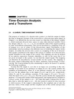
CHAPTER 3

Frequency-Domain Analysis

3.1

INTRODUCTION

In the previous chapter, we derived the definition for the z transform of a discretetime signal by impulse-sampling a continuous-time signal xa (t) with a sampling
period T and using the transformation z = esT . The signal xa (t) has another
equivalent representation in the form of its Fourier transform X(j ω). It contains
the same amount of information as xa (t) because we can obtain xa (t) from X(j ω)
as the inverse Fourier transform of X(j ω). When the signal xa (t) is sampled
with a sampling period T , to generate the discrete-time signal represented by
∞
k=0 xa (kT )δ(nT − kT ), the following questions need to be answered:
Is there an equivalent representation for the discrete-time signal in the frequency domain?
Does it contain the same amount of information as that found in xa (t)? If so,
how do we reconstruct xa (t) from its sample values xa (nT )?
Does the Fourier transform represent the frequency response of the system
when the unit impulse response h(t) of the continuous-time system is sampled? Can we choose any value for the sampling period, or is there a limit
that is determined by the input signal or any other considerations?
We address these questions in this chapter, arrive at the definition for the discretetime Fourier transform (DTFT) of the discrete-time system, and describe its properties and applications. In the second half of the chapter, we discuss another transform known as the discrete-time Fourier series (DTFS) for periodic, discrete-time
signals. There is a third transform called discrete Fourier transform (DFT), which
is simply a part of the DTFS, and we discuss its properties as well as its applications in signal processing. The use of MATLAB to solve many of the problems
or to implement the algorithms will be discussed at the end of the chapter.
Introduction to Digital Signal Processing and Filter Design, by B. A. Shenoi
Copyright © 2006 John Wiley & Sons, Inc.

112

THEORY OF SAMPLING

3.2

113

THEORY OF SAMPLING

Let us first choose a continuous-time (analog) function xa (t) that can be represented by its Fourier transform Xa (j )1
∞

Xa (j ) =

−∞

xa (t)e−j t dt

(3.1)

whereas the inverse Fourier transform of Xa (j ) is given by2
xa (t) =

∞

1
2π

−∞

Xa (j )ej t d

(3.2)

Now we generate a discrete-time sequence x(nT ) by sampling xa (t) with a
sampling period T . So we have x(nT ) = xa (t)|t=nT , and substituting t = nT in
(3.2), we can write
xa (nT ) = x(nT ) =

1
2π

∞
−∞

Xa (j )ej

nT

d

(3.3)

The z transform of this discrete-time sequence is3
∞

X(z) =

x(nT )z−n

(3.4)

n=−∞

and evaluating it on the unit circle in the z plane; thus, when z = ej ωT , we get
∞

X(ej ωT ) =

x(nT )e−j ωnT

(3.5)

n=−∞

Next we consider h(nT ) as the unit impulse response of a linear, timeinvariant, discrete-time system and the input x(nT ) to the system as ej ωnT . Then
the output y(nT ) is obtained by convolution as follows:
∞

y(nT ) =

ej ω(nT −kT ) h(kT )

k=−∞
∞

=e

j ωnT

e
k=−∞

1 The

−j ωkT

∞

h(kT ) = e

j ωnT

h(kT )e−j ωkT

(3.6)

k=−∞

material in this section is adapted from a section with the same heading, in the author’s book
Magnitude and Delay Approximation of 1-D and 2-D Digital Filters [1], with permission from the
publisher, Springer-Verlag.
2
We have chosen (measured in radians per second) to denote the frequency variable of an analog
function in this section and will choose the same symbol to represent the frequency to represent the
frequency response of a lowpass, normalized, prototype analog filter in Chapter 5.
3
Here we have used the bilateral z transform of the DT sequence, since we have assumed that it
is defined for −∞ < n < ∞ in general. But the theory of bilateral z transform is not discussed in
this book.

114

FREQUENCY-DOMAIN ANALYSIS

Note that the signal ej ωnT is assumed to have values for −∞ < n < ∞ in general, whereas h(kT ) is a causal sequence: h(kT ) = 0 for −∞ < k < 0. Hence the
−j ωkT
in (3.6) can be replaced by ∞ h(kT )e−j ωkT .
summation ∞
k=−∞ h(kT )e
k=0
j ωT
It is denoted as H (e ) and is a complex-valued function of ω, having a magnitude response H (ej ωT ) and phase response θ (ej ωT ). Thus we have the following
result
y(nT ) = ej ωnT H (ej ωT ) ej θ(e

j ωT )

(3.7)

which shows that when the input is a complex exponential function ej ωnT ,
the magnitude of the output y(nT ) is H (ej ωT ) and the phase of the output
y(nT ) is (ωnT + θ ). If we choose a sinusoidal input x(nT ) = Re(Aej ωnT ) =
A cos(ωnT ), then the output y(nT ) is also a sinusoidal function given by
y(nT ) = A H (ej ωT ) cos(ωnt + θ ). Therefore we multiply the amplitude of the
sinusoidal input by H (ej ωT ) and increase the phase by θ (ej ωT ) to get the amplitude and phase of the sinusoidal output. For the reason stated above, H (ej ωT )
is called the frequency response of the discrete-time system. We use a similar
−j ωkT
expression ∞

= X(ej ωT ) for the frequency response of any
k=−∞ x(kT )e
input signal x(kT ) and call it the discrete-time Fourier transform (DTFT) of
x(kT ).
To find a relationship between the Fourier transform Xa (j ) of the continuoustime function xa (t) and the Fourier transform X(ej ωT ) of the discrete-time
sequence, we start with the observation that the DTFT X(ej ωT ) is a periodic function of ω with a period ωs = 2π/T , namely, X(ej ωT +j rωs T ) = X(ej ωT +j r2π ) =
X(ej ωT ), where r is any integer. It can therefore be expressed in a Fourier series
form
∞

Cn e−j ωnT

(3.8)

X(ej ωT )ej ωT dω

(3.9)

X(ej ωT ) =
n=−∞

where the coefficients Cn are given by
Cn =

T
2π

π/T
−(π/T )

By comparing (3.5) with (3.8), we conclude that x(nT ) are the Fourier series
coefficients of the periodic function X(ej ωT ), and these coefficients are evaluated
from
Cn = x(nT ) =

T
2π

π/T
−(π/T )

X(ej ωT )ej ωnT dω

(3.10)

Therefore
∞

X(ej ωT ) =
n=−∞

x(nT )e−j ωnT

(3.11)


THEORY OF SAMPLING

115

Let us express (3.3), which involves integration from = −∞ to = ∞ as
the sum of integrals over successive intervals each equal to one period
2π/T = ωs :
∞

1
x(nT ) =
2π

(2r+1)π
T
(2r−1)π
T

r=−∞

Xa (j )ej

nT

d

(3.12)

However, each term in this summation can be reduced to an integral over the
range −(π/T ) to π/T by a change of variable from to + 2πr/T , to get
x(nT ) =

T
2π

∞
r=−∞

1
T

π/T
−(π/T )

Xa j

+j

2πr
T

ej

nT j 2πrn

e

d

(3.13)

Note that ej 2πrn = 1 for all integer values of r and n. By changing the order of
summation and integration, this equation can be reduced to
T

x(nT ) =
2π

π/T
−(π/T )

1
T

∞

Xa j

+j

r=−∞

2πr
T

ej

nT

Without loss of generality, we change the frequency variable
getting
x(nT ) =

T
2π

π/T
−(π/T )

1
T

∞

Xa j ω + j
r=−∞

2πr
T

d

(3.14)
to ω, thereby

ej ωnT dω

(3.15)

Comparing (3.10) with (3.15), we get the desired relationship:
X(ej ωT ) =

1
T

∞

Xa j ω + j
r=−∞

2πr
T

(3.16)

This shows that the discrete-time Fourier transform (DTFT) of the sequence
x(nT ) generated by sampling the continuous-time signal xa (t) with a sampling
period T is obtained by a periodic duplication of the Fourier transform Xa (j ω)
of xa (t) with a period 2π/T = ωs and scaled by T . To illustrate this result,
a typical analog signal xa (t) and the magnitude of its Fourier transform are
sketched in Figure 3.1. In Figure 3.2a the discrete-time sequence generated by
sampling xa (t) is shown, and in Figure 3.2b, the magnitude of a few terms of
(3.16) as well as the magnitude X(ej ωT ) are shown.
Ideally the Fourier transform of xa (t) approaches zero only as the frequency
approaches ∞. Hence it is seen that, in general, when Xa (j ω)/T is duplicated
and added as shown in Figure 3.2b, there is an overlap of the frequency responses
at all frequencies. The frequency responses of the individual terms in (3.16) add
up, giving the actual response as shown by the curve for X(ej ω ) . [We have


116

FREQUENCY-DOMAIN ANALYSIS

(a)

⎮ a( jw)⎮
X

0
(b)

Figure 3.1 An analog signal xa (t) and the magnitude of its Fourier transform X(j ω).

xa(nT)

n

0
(a)

⏐X(e jw)⏐

X(jw)
T

X( j(w − ws))
T
X( j(w − 2ws))
T

0
(b)

ws

2ws

Figure 3.2 The discrete-time signal xa (nT ) obtained from the analog signal xa (t) and
the discrete-time Fourier transform H (ej ω ).


THEORY OF SAMPLING

117

disregarded the effect of phase in adding the duplicates of X(j ω).] Because of
this overlapping effect, more commonly known as “aliasing,” there is no way of
retrieving X(j ω) from X(ej ω ) by any linear operation; in other words, we have
lost the information contained in the analog function xa (t) when we sample it.
Aliasing of the Fourier transform can be avoided if and only if (1) the function
xa (t) is assumed to be bandlimited—that is, if it is a function such that its
Fourier transform Xa (j ω) ≡ 0 for |ω| > ωb ; and (2) the sampling period T is
chosen such that ωs = 2π/T > 2ωb . When the analog signal xb (t) is bandlimited
as shown in Figure 3.3b and is sampled at a frequency ωs ≥ 2ωb , the resulting
discrete-time signal xb (nT ) and its Fourier transform X(ej ω ) are as shown in
Figure 3.4a,b, respectively.
If this bandlimited signal xb (nT ) is passed through an ideal lowpass filter
with a bandwidth of ωs /2, the output will be a signal with a Fourier transform
equal to X(ej ωT )Hlp (j ω) = Xb (j ω)/T . The unit impulse response of the ideal
lowpass filter with a bandwidth ωb obtained as the inverse Fourier transform of
Hlp (j ω) is given by
hlp (t) =

1
2π

1
=
2π
sin
=

∞
−∞

Hlp (j ω)ej ωt dω

ωs
2
−ωs
2

T ej ωt dω

ωs t
2
ωs t
2

sin
=

(3.17)
πt
T

πt
T

(3.18)

xb(t )

0

t
(a)
⏐ b( jw)⏐
X

−wb

wb
(b)

Figure 3.3 A bandlimited analog signal and the magnitude of its Fourier transform.


118

FREQUENCY-DOMAIN ANALYSIS

xb(nT )

0

n
(a)
Ideal analog lowpass filter

−

wt
−wb
2

wb

wt
2

wt

(b)

Figure 3.4 The discrete-time signal obtained from the bandlimited signal and the magnitude of its Fourier transform.

The output signal will be the result of convolving the discrete input sequence
xb (nT ) with the unit impulse response hlp (t) of the ideal analog lowpass filter. But we have not defined the convolution between a continuous-time signal
and samples of discrete-time sequence. Actually it is the superposition of the
responses due to the delayed impulse responses hlp (t − nT ), weighted by the
samples xb (nT ), which gives the output xb (t). Using this argument, Shannon [2]
derived the formula for reconstructing the continuous-time function xb (t), from
only the samples x(n) = xb (nT )—under the condition that xb (t) be bandlimited
up to a maximum frequency ωb and be sampled with a period T < π/ωb . This
formula (3.19) is commonly called the reconstruction formula, and the statement

that the function xb (t) can be reconstructed from its samples xb (nT ) under the
abovementioned conditions is known as Shannon’s sampling theorem:
∞

xb (t) =

sin
xb (nT )

n=−∞

π
(t − nT )
T
π
(t − nT )
T

(3.19)

The reconstruction process is indicated in Figure 3.5a. An explanation of the
reconstruction is also given in Figure 3.5b, where it is seen that the delayed
π
π
impulse response sin T (t − nT ) / T (t − nT ) has a value of xb (nT ) at t = nT
and contributes zero value at all other sampling instants t = nT so that the
reconstructed analog signal interpolates exactly between these sample values of
the discrete samples.

THEORY OF SAMPLING

119

Ideal Lowpass analog filter hf(t )

xb (nT )

xb(t ) = xb(nT )∗hf(t )

Hf( jw)

Xb(jw) = Xb(e jwT)Hf(jw)

Xb(e jωT)

(a)
x(0)

Reconstructed signal
x(T)

−T

0

T

2T
(b)

3T

4T

Figure 3.5 Reconstruction of the bandlimited signal from its samples, using an ideal
lowpass analog filter.

This revolutionary theorem implies that the samples xb (nT ) contain all the
information that is contained in the original analog signal xb (t), if it is bandlimited and if it has been sampled with a period T < π/ωb . It lays the necessary
foundation for all the research and developments in digital signal processing
that is instrumental in the extraordinary progress in the information technology
that we are witnessing.4 In practice, any given signal can be rendered almost
bandlimited by passing it through an analog lowpass filter of fairly high order.
Indeed, it is common practice to pass an analog signal through an analog lowpass
filter before it is sampled. Such filters used to precondition the analog signals
are called as antialiasing filters. As an example, it is known that the maximum
frequency contained in human speech is about 3400 Hz, and hence the sampling
frequency is chosen as 8 kHz. Before the human speech is sampled and input to
telephone circuits, it is passed through a filter that provides an attenuation of at
least 30 dB at 4000 Hz. It is obvious that if there is a frequency above 4000 Hz
in the speech signal, for example, at 4100 Hz, when it is sampled at 4000 Hz,
due to aliasing of the spectrum of the sampled signal, there will be a frequency
at 4100 Hz as well as 3900 Hz. Because of this phenomenon, we can say that
the frequency of 4100 Hz is folded into 3900 Hz, and 4000 Hz is hence called
the “folding frequency.” In general, half the sampling frequency is known as the
folding frequency (expressed in radians per second or in hertz).
4
This author feels that Shannon deserved an award (such as the Nobel prize) for his seminal contributions to sampling theory and information theory.

120

FREQUENCY-DOMAIN ANALYSIS

There is some ambiguity in the published literature regarding the definition of
what is called the Nyquist frequency. Most of the books define half the sampling
frequency as the Nyquist frequency and 2fb as the Nyquist rate, which is the
minimum sampling rate required to avoid aliasing. Because of this definition for
the Nyquist rate, some authors erroneously define fb as the Nyquist frequency.
In our example, when the signal is sampled at 8 kHz, we have 4 kHz as the
Nyquist frequency (or the folding frequency) and 6.8 kHz as the Nyquist rate.
If we sample the analog signal at 20 kHz, the Nyquist frequency is 10 kHz, but
the Nyquist rate is still 6.8 kHz. We will define half the sampling frequency as
the Nyquist frequency throughout this book. Some authors define the Nyquist
frequency as the bandwidth of the corresponding analog signal, whereas some
authors define 2fb as the bandwidth.
3.2.1

Sampling of Bandpass Signals

Suppose that we have an analog signal that is a bandpass signal (i.e., it has a
Fourier transform that is zero outside the frequency range ω1 ≤ ω ≤ ω2 ); the
bandwidth of this signal is B = ω2 − ω1 , and the maximum frequency of this
signal is ω2 . So it is bandlimited, and according to Shannon’s sampling theorem,
one might consider a sampling frequency greater than 2ω2 ; however, it is not
necessary to choose a sampling frequency ωs ≥ 2ω2 in order to ensure that we
can reconstruct this signal from its sampled values. It has been shown [3] that
when ω2 is a multiple of B, we can recover the analog bandpass signal from its
samples obtained with only a sampling frequency ωs ≥ 2B. For example, when

the bandpass signal has a Fourier transform between ω1 = 4500 and ω2 = 5000,
we don’t have to choose ωs > 10,000. We can choose ωs > 1000, since ω2 =
10B in this example.
Example 3.1

Consider a continuous-time signal xa (t) = e−0.2t u(t) that has the Fourier
transform X(j ω) = 1/(j ω + 0.2). The magnitude |X(j ω)| = |1/(j ω + 0.2)| =
1/(ω2 + 0.04), and when we choose a frequency of 200π, we see that the
magnitude is approximately 0.4(10−3 ). Although the function xa (t) = e−0.2t u(t)
is not bandlimited, we can assume that it is almost bandlimited with bandwidth
of 200π and choose a sampling frequency of 400π rad/s or 200 Hz. So the sam1
pling period T = 200 = 0.005 second and ωs = 2π/T = 400π rad/s. To verify
that (3.11) and (3.16) both give the same result, let us evaluate the DTFT at
ω = 0.5 rad/s. According to (3.11), the DTFT of x(nT ) is
∞
n=0

e−0.2(nT ) e−j ωnT =

∞

e−0.001n e−j ωn(0.005)

n=0

= X(ej ωT ) =

1
1 − e−0.001 e−j (0.005ω)

(3.20)


THEORY OF SAMPLING

121

and its magnitude at ω = 0.5 is
1
1−

e−0.001 e−j (0.0025)

= 371.5765

According to (3.16), the DTFT for this example becomes
1
0.005

∞
k=−∞

1
0.2 + j (ω + k400π)

(3.21)

and at ω = 0.5, we can neglect the duplicates at j k400π and give the magnitude
of the frequency response as
1

1
= 371.3907
0.005 0.2 + j 0.5
The two magnitudes at ω = 0.5 are nearly equal; the small difference is
attributable to the slight aliasing in the frequency response. See Figure 3.6, which
illustrates the equivalence of the two equations. But (3.16) is not useful when
a sequence of arbitrary values (finite or infinite in length) is given because it
is difficult to guess the continuous-time signal of which they are the sampled
values; even if we do know the continuous-time signal, the choice of a sampling
frequency to avoid aliasing may not be practical, for example, when the signal is
a highpass signal. Hence we refer to (3.11) whenever we use the acronym DTFT
in our discussion.

X(jw)

0

200 p

X(e jw)

0

200 p

fs = 400p

w

Figure 3.6 Equivalence of the two definitions for the Fourier transform of a discrete-time

signal.


122

3.3

FREQUENCY-DOMAIN ANALYSIS

DTFT AND IDTFT

The expressions for the DTFT X(ej ω ) and the IDTFT x(n) are
∞
jω

X(e ) =

x(n)e−j ωn

(3.22)

n=0

x(n) =

1
2π

π
−π

X(ej ω )ej ωn dω

(3.23)

The DTFT and its inverse (IDTFT) are extensively used for the analysis and
design of discrete-time systems and in applications of digital signal processing
such as speech processing, speech synthesis, and image processing. Remember
that the terms frequency response of a discrete-time signal and the discrete-time
Fourier transform (DTFT) are synonymous and will be used interchangeably.
This is also known as the frequency spectrum; its magnitude response and
phase response are generally known as the magnitude spectrum and phase spectrum, respectively. We will also use the terms discrete-time signal, discrete-time
sequence, discrete-time function, and discrete-time series synonymously.
We will represent the frequency response of the digital filter either by
H (ej ωT ) or more often by H (ej ω ) for convenience. Whenever it is expressed
as H (ej ω )—which is very common practice in the published literature—the
frequency variable ω is to be understood as the normalized frequency ωT =
ω/fs . We may also represent the normalized frequency ωT by θ (radians). In
Figure 3.7a, we have shown the magnitude response of an ideal lowpass filter,
demonstrating that it transmits all frequencies from 0 to ωc and rejects frequencies
higher than ωc . The frequency response H (ej ω ) is periodic, and its magnitude is
an even function. In Figure 3.7b suppose we have shown the magnitude response
of the lowpass filter only over the frequency range [0 π]. We draw its magnitude for negative values of ω since it is an even function and extend it by repeated
duplication with a period of 2π, thereby obtaining the magnitude response for all
values of ω over the range (−∞, ∞). Therefore, if the frequency specifications
are given over the range [0 π], we know the specifications for all values of the
normalized frequency ω, and the specifications for digital filters are commonly
given for only this range of frequencies. Note that we have plotted the magnitude response as a function of the normalized frequency ω. Therefore the range
[0 π] corresponds to the actual frequency range [0 ωs /2] and the normalized
frequency π corresponds to the Nyquist frequency (and 2π corresponds to the

sampling frequency).
Sometimes the frequency ω is even normalized by πfs so that the Nyquist
frequency has a value of 1, for example, in MATLAB functions. In Figures 3.7c,d,
we have shown the magnitude response of an ideal highpass filter. In Figure 3.8
we show the magnitude responses of an ideal bandpass and bandstop filter.
It is convenient to do the analysis and design of discrete-time systems on
the basis of the normalized frequency. When the frequency response of a filter, for example, shows a magnitude of 0.5 (i.e., −6 dB) at the normalized


DTFT AND IDTFT

123

⎮ lp(e jw)
H
⎮
l

−2p

−p −wc

wc

0

p

2p

2w

(a)
⎮
⎮ lp(e jw)
H

−p −wc

wc

0

p

(b)
⎮ lp(e jw)
H
⎮

−2p

−p

−wc

0

wc

p

2p

w

(c)
⎮ lp(e jw)
H
⎮

0

wc

p

w

(d)

Figure 3.7 Magnitude responses of ideal lowpass and highpass filters.

frequency 0.3π, the actual frequency can be easily computed as 30% of the
Nyquist frequency, and when the sampling period T or the sampling frequency
ωs (or fs = 1/T ) is given, we know that 0.3π represents (0.3)(ωs /2) rad/s or
(0.3)(fs /2) Hz. By looking at the plot, one should therefore be able to determine
what frequency scaling has been chosen for the plot. And when the actual sampling period is known, we know how to restore the scaling and find the value
of the actual frequency in radians per second or in hertz. So we will choose the
normalized frequency in the following sections, without ambiguity.

The magnitude response of the ideal filters shown in Figures 3.7 and 3.8 cannot
be realized by any transfer function of a digital filter. The term “designing a digital
filter” has different meanings depending on the context. One meaning is to find a
transfer function H (z) such that its magnitude H (ej ω ) approximates the ideal
magnitude response as closely as possible. Different approximation criteria have
been proposed to define how closely the magnitude H (ej ω ) approximates the
ideal magnitude. In Figure 3.9a, we show the approximation of the ideal lowpass
filter meeting the elliptic function criteria. It shows an error in the passband as


124

FREQUENCY-DOMAIN ANALYSIS

⎮ bp(e jw)
H
⎮

0

wc2 π

wc1

w

(a)
⎮
⎮ bs(e jw)
H

0

wc1 wc2

π

w

(b)

Figure 3.8 Magnitude responses of ideal bandpass and bandstop filters.

Magnitude response of elliptic lowpass filter
1
Passband

Magnitude

0.8
0.6
0.4

Transition band
Stopband

0.2
0

0

0.1

0.2

0.3

0.4
0.5
0.6
0.7
Normalized frequency w/pi
(a)

0.8

0.9

1

0.9

1

Magnitude response of Butterworth highpass filter
1.4

Magnitude

1.2

1
0.8
Passband

0.6
0.4
0.2
0

Stopband
0

0.1

0.2

0.3

0.4

0.5

0.6

0.7

0.8

Normalized frequency w/pi
(b)

Figure 3.9 Approximation of ideal lowpass and highpass filter magnitude response.


DTFT AND IDTFT

125

Magnitude response of Chebyshev I bandpass filter
1
Passband

Magnitude

0.8
0.6
0.4
0.2
0

0

Stopband
0.1
0.2

0.3

0.4

0.5

0.6

Stopband
0.7
0.8

0.9

1

0.9

1

Normalized frequency w/pi
(a)
Magnitude response of Chebyshev II bandstop filter
1.4

Magnitude

1.2
1

Passband

Passband

0.8
0.6
0.4
0.2
0

Stopband
0

0.1

0.2

0.3

0.4

0.5

0.6

0.7

0.8

Normalized frequency w/pi
(b)

Figure 3.10

Approximation of ideal bandpass and bandstop digital filters.

well as in the stopband, which is equiripple in nature, whereas in Figure 3.9b,
the magnitude of a highpass filter is approximated by a Butterworth type of
approximation, which shows that the magnitude in the passband is “nearly flat”
and decreases monotonically as the frequency decreases from the passband.
Figure 3.10a illustrates a Chebyshev type I approximation of an ideal bandpass filter, which has an equiripple error in the passband and a monotonically
decreasing response in the stopband, whereas in Figure 3.10b, we have shown a
Chebyshev type II approximation of an ideal bandstop filter; thus, the error in
the stopband is equiripple in nature and is monotonic in the passband. The exact
definition of these criteria and the design of filters meeting these criteria will be
discussed in the next two chapters.
3.3.1

Time-Domain Analysis of Noncausal Inputs

Let the DTFT of the input signal x(n) and the unit impulse response h(n) of
a discrete-time system be X(ej ω ) and H (ej ω ), respectively. The output y(n)
is obtained by the convolution sum x(n) ∗ h(n) = y(n) = ∞
k=−∞ h(k)x(n − k),
which shows that the convolution sum is applicable even when the input signal


126

FREQUENCY-DOMAIN ANALYSIS

is defined for −∞ < n < 0 or −∞ < n < ∞. In this case, the unilateral z transform of x(n) cannot be used. Therefore we cannot find the output y(n) as the
inverse z transform of X(z)H (z). However, we can find the DTFT of the input
sequence even when it is defined for −∞ < n < ∞, and then multiply it by the

DTFT of h(n) to get the DTFT of the output as Y (ej ω ) = X(ej ω )H (ej ω ). Its
IDTFT yields the output y(n). This is one advantage of using the discrete-time
Fourier transform theory. So for time-domain analysis, we see that the DTFTIDTFT pair offers an advantage over the z-transform method, when the input
signal is defined for −∞ < n < 0 or −∞ < n < ∞. An example is given later
to illustrate this advantage over the z-transform theory in such cases.
The relationship Y (ej ω ) = X(ej ω )H (ej ω ) offers a greater advantage as it is
the basis for the design of all digital filters. When we want to eliminate certain
frequencies or a range of frequencies in the input signal, we design a filter such
that the magnitude of H (ej ω ) is very small at these frequencies or over the
range of frequencies that would therefore form the stopband. The magnitude of
the frequency response H (ej ω ) at all other frequencies is maintained at a high
level, and these frequencies constitute the passband. The magnitude and phase
responses of the filter are chosen so that the magnitude and phase responses of
the output of the filter will have an improved quality of information. We will
discuss the design of digital filters in great detail in Chapters 4 and 5. We give
only a simple example of its application in the next section.
Example 3.2

Suppose that the input signal has a lowpass magnitude response with a bandwidth
of 0.7π as shown in Figure 3.11 and we want to filter out all frequencies outside
the range between ω1 = 0.3π and ω2 = 0.4π. Note that the sampling frequency
of both signals is set at 2π. If we pass the input signal through a bandpass
filter with a passband between ω1 = 0.3π and ω2 = 0.4π, then the frequency
response of the output is given by a bandpass response with a passband between
ω1 = 0.3π and ω2 = 0.4π, with all the other frequencies having been filtered
out. It is interesting to observe that the maximum frequency in the output is
0.4π; therefore, we can reconstruct y(t) from the samples y(n) and then sample
at a lower sampling frequency of 0.8π, instead of the original frequency of 2π.
If the sampling frequency in this example is 10,000 Hz, then the Nyquist frequency is 5000 Hz, and therefore the input signal has a bandwidth of 3500 Hz,
corresponding to the normalized bandwidth of 0.7π, whereas the bandpass filter

has a passband between 1500 and 2000 Hz. The output of the bandpass filter has
a passband between 1500 and 2000 Hz. Since the maximum frequency in the
output signal is 2000 Hz, one might think of reconstructing the continuous-time
signal using a sampling frequency of 4000 Hz. But this is a bandpass signal
with a bandwidth of 500 Hz, and 2000 Hz is 8 times the bandwidth; according
to the sampling theorem for bandpass signals, we can reconstruct the output signal y(t) using a sampling frequency of twice the bandwidth, namely, 1000 Hz
instead of 4000 Hz. The theory and the procedure for reconstructing the analog


DTFT AND IDTFT

|Xlp(e jw)|

127

|Hbp(e jw)|
5

3

0

0.7π

π

0

π

w

0.3π 0.4π

|X(e jw)|
15

0

0.3π 0.4π

w

π

Figure 3.11 A lowpass signal processed by a bandpass filter.

bandpass signal from its samples is beyond the scope of this book and will not
be treated further.
3.3.2

Time-Shifting Property

If x(n) has a DTFT X(ej ω ), then x(n − k) has a DTFT equal to e−j ωk X(ej ω ),
where k is an integer. This is known as the time-shifting property and it
−j ωn
is easily proved as follows: DTFT of x(n − k) = ∞
=
n=−∞ x(n − k)e
∞

−j ωk
−j ωn = e−j ωk X(ej ω ). So we denote this property by
x(n)e
e
n=−∞
x(n − k) ⇔ e−j ωk X(ej ω )
3.3.3

Frequency-Shifting Property

If x(n) ⇔ X(ej ω ), then
ej ω0 n x(n) ⇔ X(ej (ω−ω0 ) )
This is known as the frequency-shifting property, and it is easily proved as
follows:
∞
n=−∞

x(n)ej ω0 n e−j ωn =

∞
n=−∞

x(n)e−j (ω−ω0 )n = X(ej (ω−ω0 ) )


128

FREQUENCY-DOMAIN ANALYSIS

3.3.4

Time Reversal Property

Let us consider x(n) = a n u(n). Its DTFT X(ej ω ) = ∞ a n e−j ωn . Next, to find
n=0
the DTFT of x(−n), if we replace n by −n, we would write the DTFT of x(−n)
as −∞ a −n ej ωn (but that is wrong), as illustrated by the following example:
n=0
∞

X(ej ω ) =

a n e−j ωn = 1 + ae−j ω + a 2 e−j 2ω + a 3 e−j 3ω + · · ·

n=0

But the correct expression for the DTFT of x(−n) is of the form 1 + aej ω +
a 2 ej 2ω + a 3 ej 3ω + · · · .
−n −j ωn . With this clarificaSo the compact form for this series is 0
n=−∞ a e
tion, we now prove the property that if x(n) ⇔ X(ej ω ) then
x(−n) ⇔ X(e−j ω )

(3.24)

−j ωn . We substitute (−n) = m, and
Proof : DTFT of x(−n) = ∞
n=−∞ x(−n)e
∞
∞

−j ωn
−j (−ω)m
we get
= m=−∞ x(m)ej ωm = ∞
=
n=−∞ x(−n)e
m=−∞ x(m)e
−j ω
).
X(e

Example 3.3

Consider x(n) = δ(n). Then, from the definition for DTFT, we see that δ(n) ⇔
X(ej ω ) = 1 for all ω.
From the time-shifting property, we get
δ(n − k) ⇔ e−j ωk

(3.25)

The Fourier transform e−j ωk has a magnitude of one at all frequencies but a
linear phase as a function of ω that yields a constant group delay of k samples. If
we extend this result by considering an infinite sequence of unit impulses, which
∞
−j ωk
can be represented by ∞
.
k=−∞ δ(n − k), its DTFT would yield
k=−∞ e
But this does not converge to any form of expression. Hence we resort to a

different approach, as described below, and derive the result (3.28).
Example 3.4

We consider x(n) = δ(n + k) + δ(n − k). Its DTFT is given by X(ej ω ) = ej ωk +
e−j ωk = 2 cos(ωk). In this example, note that the DTFT is a function of the
continuous variable ω whereas k is a fixed number. It is a periodic function of
ω with a period of 2π, because 2 cos((ω + 2rπ)k) = 2 cos(ωk), where r is an
integer. In other words, the inverse DTFT of X(ej ω ) = 2 cos(ωk) is a pair of
impulse functions at n = k and n = −k, and this is given by
cos(ωk) ⇔ 1 [δ(n + k) + δ(n − k)]
2

(3.26)


DTFT AND IDTFT

129

Example 3.5

Now we consider the infinite sequence of x(n) = 1 for all n. We represent it in
the form x(n) = ∞
k=−∞ δ(n − k). We prove below that its DTFT is given as
2π ∞
δ(ω − 2πk), which is a periodic train of impulses in the frequency
k=−∞
domain, with a strength equal to 2π and a period equal to 2π (which is the
normalized sampling frequency). We prove this result given by (3.27), by showing
that the inverse DTFT of 2π ∞

k=−∞ δ(ω − 2πk) is equal to one for all n.
∞

δ(ω − 2πk) ⇔ 1 (for all n)

2π

(3.27)

k=−∞

Proof : The inverse DTFT of 2π

δ(ω − 2πk) ej ωn dω

2π

−π

k=−∞

π

∞

−π

=

δ(ω − 2πk) is evaluated as

∞

π

1
2π

∞
k=−∞

k=−∞

δ(ω − 2πk) ej ωn dω

From the sifting property we get
∞

∞

δ(ω − 2πk) ej ωn =

δ(ω − 2πk) ej 2πkn

k=−∞

k=−∞
∞

=

δ(ω − 2πk)
k=−∞

where we have used ej 2πkn = 1 for all n. When we integrate the sequence of
impulses from −π to π, we have only the impulse at ω = 0.
Therefore
π

∞

−π

k=−∞

δ(ω − 2πk) ej ωn dω

=

π

∞

−π k=−∞

δ(ω)ej ωn dω = 1

(for all n)

Thus we have derived the important result

∞

∞

δ(n − k) ⇔ 2π
k=−∞

δ(ω − 2πk)
k=−∞

(3.28)


130

FREQUENCY-DOMAIN ANALYSIS

To point out some duality in the results we have obtained above, let us repeat
them:
When x(n) = 1 at n = 0 and 0 at n = 0, that is, when we have δ(n), its DTFT
X(ej ω ) = 1 for all ω.
When x(n) = 1 for all n, specifically, when we have ∞
k=−∞ δ(n − k), its
δ(ω − 2πk).
DTFT X(ej ω ) = 2π ∞
k=−∞
Using the frequency-shifting property, we get the following results:
∞

ej ω0 n ⇔ 2π

δ(ω − ω0 − 2πk)

(3.29)

k=−∞

From these results, we can obtain the DTFT for the following sinusoidal
sequences:
∞

cos(ω0 n) =

1 j ω0 n
[e
+ e−j ω0 n ] ⇔ π
δ(ω − ω0 − 2πk) + δ(ω + ω0 − 2πk)
2
k=−∞

sin(ω0 n) =

1 j ω0 n −j ω0 n
π
[e
−e
]⇔
δ(ω − ω0 − 2πk) − δ(ω + ω0 − 2πk)
2j
j k=−∞

∞

(3.30)
Now compare the results in (3.28) and (3.30), which are put together in (3.31)
and (3.32) in order to show the dualities in the properties of the two transform
pairs. Note in particular that cos(ωk) is a discrete-time Fourier transform and a
function of ω, where k is a fixed integer, whereas cos(ω0 n) is a discrete-time
sequence where ω0 is fixed and is a function of n:
1
2 [δ(n

+ k) + δ(n − k)] ⇐⇒ cos(ωk)

(3.31)

∞

cos(ω0 n) ⇐⇒ π

δ(ω − ω0 − 2πk) + δ(ω + ω0 − 2πk)
k=−∞

(3.32)
Let us show the duality of the other functions derived in (3.26) and (3.29)
δ(n) ⇐⇒ 1

for all ω

whereas

∞

x(n) = 1 for all n ⇐⇒ 2π

δ(ω − 2πk)
k=−∞


DTFT AND IDTFT

131

Using the time- and frequency-shifting properties on these functions, we
derived the following Fourier transform pairs as well:
δ(n − k) ⇐⇒ e−j ωk
∞

e

j ω0 n

⇐⇒ 2π

δ(ω − ω0 − 2πk)
k=−∞

Example 3.6

This is another example chosen to highlight the difference between the
expressions for the discrete-time sequence x(n) and its DTFT X(ej ω ). So if

we are given F (ej ω ) = 10 cos(5ω) + 5 cos(2ω) = 5ej 5ω + 5e−j 5ω + 2.5ej 2ω +
2.5e−j 2ω , its IDTFT is obtained by using the result δ(n − k) ⇔ e−j ωk , and we
get f (n) = 5δ(n + 5) + 2.5δ(n + 2) + 2.5δ(n − 2) + 5δ(n − 5), which is plotted in Figure 3.12a. Obviously it is a finite sequence with four impulse functions
and therefore is not periodic.
f(n)
5

2.5

−5 −4 −3 −2 −1 0

1 2 3 4 5
(a)

n

|G(e jw)|
10

5

−0.5π

−0.2π

0.2π

0

0.5π

w

(b)

Figure 3.12 A sequence of impulses in the discrete-time domain and a sequence of
impulses in the discrete-frequency domain.


132

FREQUENCY-DOMAIN ANALYSIS

If we are given a function g(n) = 10 cos(0.5πn) + 5 cos(0.2πn), the first thing
we have to recognize is that it is a discrete-time function and is a periodic function
in its variable n. So we find its DTFT, using (3.30), as
∞

G(ej ω ) = 10π

∞

δ(ω − 0.5π − 2πk) + 10π
k=−∞

δ(ω + 0.5π − 2πk)
k=−∞

∞

+ 5π

∞

δ(ω − 0.2π − 2πk) + 5π
k=−∞

δ(ω + 0.2π − 2πk)
k=−∞

This DTFT is shown in Figure 3.12b. We notice that it represents an infinite
number of impulses in the frequency domain that form a periodic function in the
frequency variable ω. Because it has discrete components, the impulse functions
are also called the spectral components of g(n).
We have chosen a DTFT F (ej ω ) and derived its IDTFT f (n), which is a
sequence of impulse functions in the time domain as shown in Figure 3.12a;
then we chose a discrete-time function g(n) and derived its DTFT G(ej ω ),
which is a sequence of impulse functions in the frequency domain as shown
in Figure 3.12b.
Example 3.7

Consider the simple example of a discrete-time sinsusoidal signal x(n) =
4 cos(0.4πn). It is periodic when the frequency (0.4N ) is an integer or a ratio of
integers. We choose N = 5 as the period of this function, so x(n) = x(n + 5K) =
4 cos[0.4π(n + 5K)], where K is any integer.
We rewrite x(n) = 2[ej 0.4πn + e−j 0.4πn ], and therefore its DTFT X(ej ω ) =
∞
2π ∞
k=−∞ δ(ω − 0.4π − 2πk) + 2π
k=−∞ δ(ω + 0.4π − 2πk). It consists of

impulse functions of magnitude equal to 2π, at ω = ±(0.4π + 2πK) in the
frequency domain and with a period of 2π.
Given f (n) = 2δ(n + 4) + 2δ(n − 4), its DTFT is F (ej ω ) = 4 cos(4ω), and
if x(n) = 4 cos(0.4πn), its DTFT is X(ej ω ) = 2π ∞
k=−∞ δ(ω − 0.4π − 2πk) +
2π ∞
δ(ω + 0.4π − 2πk).
k=−∞
Examples 3.6 and 3.7 have been chosen in particular to distinguish the differences between the two Fourier transform pairs.
Example 3.8

Let us consider the DTFT of some more sequences. For example, the DTFT of
x1 (n) = a n u(n) is derived below:
∞

X1 (ej ω ) =
n=0

a n e−j ωn =

∞
n=−∞

ae−j ω

n


DTFT AND IDTFT

133

This infinite series converges to 1/(1 − ae−j ω ) = ej ω /(ej ω − a) when
ae−j ω < 1, that is, when |a| < 1. So, the DTFT of (0.4)n u(n) is 1/(1 − 0.4e−j ω )
and the DTFT of (−0.4)n u(n) is 1/(1 + 0.4e−j ω ). Note that both of them are causal
sequences.
If we are given a sequence x13 (n) = a |n| , where |a| < 1, we split the sequence
as a causal sequence x1 (n) from 0 to ∞, and a noncausal sequence x3 (n)
from −∞ to −1. In other words, we can express x1 (n) = a n u(n) and x3 (n) =
a −n u(−n − 1). We derive the DTFT of x13 (n) as
∞

X13 (ej ω ) =

a n e−j ωn +

−1

a −n e−j ωn X1 (ej ω ) + X3 (ej ω )

n=−∞

n=0

Substituting m = −n in the second summation for X3 (ej ω ), we get
∞

X13 (ej ω ) =

ae−j ω

n

n=0
∞

=

∞

+

aej ω

m

m=1

ae−j ω

n

∞

−1+

n=0

aej ω

m

m=0

=

1
1
−1+
−j ω
1 − ae
1 − aej ω

=

aej ω
1
+
1 − ae−j ω
1 − aej ω

=

1 − a2
1 − 2a cos ω + a 2

for |a| < 1

for |a| < 1

Hence we have shown that
a |n| ⇔

1 − a2
1 − 2a cos ω + a 2

for |a| < 1

These results are valid when |a| < 1. From the result a n u(n) ⇔ 1/(1 − ae−j ω ),
by application of the time-reversal property, we also find that x4 (n) = x1 (−n) =
a −n u(−n) ⇔ 1/(1 − aej ω ) for |a| < 1 whereas we have already determined that
x3 (n) = a −n u(−n − 1) ⇔ aej ω /(1 − aej ω ). Note that x3 (n) is obtained from
x4 (n) by deleting the sample of x4 (n) at n = 0, specifically, x4 (n) − 1 = x3 (n).
We used this result in deriving X3 (ej ω ) above. The sequence x13 (n) is plotted in
Figure 3.13, while the plots of x1 (n), x3 (n) are shown in Figures 3.14 and 3.15,
respectively.


134

FREQUENCY-DOMAIN ANALYSIS

x13(n)

−8

−7

−6

−5

−4

−3

−2

−1

0

1

2

3

4

5

6

7

8

n

Figure 3.13 The discrete-time sequence x13 (n).

x1(n)
1.0
0.8
0.64
0.512
0.41
0.328
0.262

0

1

2

3

4

5

6

0.21

7

0.168

8

n

Figure 3.14 The discrete-time sequence x1 (n).

x3(n)

0.8
0.64
0.512
0.41
0.328
0.262
0.168

−7

−6

−5

−4

−3

−2

−1

0

Figure 3.15 The discrete-time sequence x3 (n).

n

0.134


DTFT AND IDTFT

135

x5(n)

0.5

0.25
0.125
0.0315 0.0625
−7

−6

−5

−4

−3

−2

−1

0

2 n

1

Figure 3.16 The discrete-time sequence x5 (n).

Now let us consider the case of x5 (n) = α n u[−(n + 1)], where |α| > 1. A plot
of this sequence is shown in Figure 3.16 for α = 2. Its DTFT is derived below:
∞

α n u[−(n + 1)]e−j ωn

X5 (ej ω ) =
n=−∞
−∞

n

αe−j ω

=

−∞

1 jω
e
α

=

n=−1

n=−1

−n

By a change of variable n = −m, we get
∞

X5 (e ) =
m=1

= −1 +
=

∞

m

1 jω
e
α

jω

= −1 +
m=0

1 jω
e
α

m

1
1−

1 jω
αe

1
αe−j ω

−1

So we have the transform pair
x5 (n) = α n u[−(n + 1)] ⇔

1
αe−j ω − 1

=

ej ω
α − ej ω

when |α| > 1

(3.33)

It is important to exercise caution in determining the differences in this pair
(3.33), which is valid for |α| > 1, and the earlier pairs, which are valid for |a| < 1.
All of them are given below (again, the differences between the different DTFTIDTFT pairs and the corresponding plots should be studied carefully and clearly
understood):
x1 (n) = a n u(n) ⇔

1
ej ω
= jω
1 − ae−j ω
e −a

when |a| < 1

(3.34)


136

FREQUENCY-DOMAIN ANALYSIS

x4 (n) = a −n u(−n) ⇔

1
e−j ω
= −j ω
1 − aej ω
e
−a

when |a| < 1

(3.35)

aej ω
1 − aej ω

when |a| < 1

(3.36)

1 − a2
1 − 2a cos ω + a 2

when |a| < 1

(3.37)

x3 (n) = a −n u(−n − 1) ⇔
x13 (n) = x1 (n) + x3 (n) ⇔

For the sequence x5 (n) = α n u[−(n + 1)], note that the transform pair is given
by (3.38), which is valid when |α| > 1:

x5 (n) = α n u[−(n + 1)] ⇔

1
αe−j ω

−1

=

ej ω
α − ej ω

when |α| > 1

(3.38)

Example 3.9

A few examples are given below to help explain these differences. From the
results given above, we see that
1. If the DTFT X1 (ej ω ) = 1/(1 − 0.8e−j ω ), its IDTFT is x1 (n) = (0.8)n u(n).
2. The IDTFT of X3 (ej ω ) = 0.8ej ω /(1 − 0.8ej ω ) is given by x3 (n) =
(0.8)−n [u(−n − 1)].
3. The IDTFT of X4 (ej ω ) = 1/(1 − 0.8ej ω ) is x4 (n) = (0.8)−n u(−n). But
4. The IDTFT of X5 (ej ω ) = ej ω /(2 − ej ω ) is x5 (n) = (2)n u(−n − 1).
Note the differences in the examples above, particularly the DTFT-IDTFT pair
for x5 (n).
The magnitude and phase responses of X1 (ej ω ), X3 (ej ω ), and X13 (ej ω ) are
shown in Figures 3.17, 3.18, and 3.19, respectively. The magnitude responses of
X1 (ej ω ), X4 (ej ω ), and X3 (ej ω ) given below appear the same except for a scale

5

4.5

4

4

3

3.5

2

3

1

2.5

0
−2

−1

0

1

2

2
−2

−1

0

Figure 3.17 The magnitude and phase responses of x1 (n).

1

2