Design And Analysis Of Dynamic Huffman Codes

Design and Analysis of Dynamic Huffman Codes
JEFFREY SCOTT VITTER
Brown University, Providence, Rhode Island
Abstract. A new one-pass algorithm for constructing dynamic Huffman codes is introduced and
analyzed. We also analyze the one-pass algorithm due to Failer, Gallager, and Knuth. In each algorithm,
both the sender and the receiver maintain equivalent dynamically varying Huffman trees, and the
coding is done in real time. We show that the number of bits used by the new algorithm to encode a
message containing t letters is < t bits more than that used by the conventional two-pass Huffman
scheme, independent of the alphabet size. This is best possible in the worst case, for any one-pass
Huffman method. Tight upper and lower bounds are derived. Empirical tests show that the encodings
produced by the new algorithm are shorter than those of the other one-pass algorithm and, except for
long messages,are shorter than those of the two-pass method. The new algorithm is well suited for online encoding/decoding in data networks and for file compression.
Categories and Subject Descriptors: C.2.0 [Computer-Communication Networks]: General-data communications; E.1 [Data]: Data Structures-trees; E.4 [Data]: Coding and Information Theory-data
compaction and compression; nonsecret encoding schemes; F.2.2 [Analysis of Algorithms and Problem
Complexity]: Nonnumerical Algorithms and Problems; G.2.2 [Discrete Mathematics]: Graph Theorytrees; H. 1.I [Models and Principles]: Systems and Information Theory-value of information
General Terms: Algorithms, Design, Performance, Theory
Additional Key Words and Phrases: Distributed computing, entropy, Huffman codes

1. Introduction
Variable-length source codes, such as those constructed by the well-known twopass algorithm due to D. A. Huffman [5], are becoming increasingly important for
several reasons. Communication costs in distributed systems are beginning to
dominate the costs for internal computation and storage. Variable-length codes
often use fewer bits per source letter than do fixed-length codes such as ASCII and
EBCDIC, which require rlog nl bits per letter, where n is the alphabet size. This
can yield tremendous savings in packet-based communication systems. Moreover,
Support was provided in part by National Science Foundation research grant DCR-84-03613, by an
NSF Presidential Young Investigator Award with matching funds from an IBM Faculty Development
Award and an AT&T research grant, by an IBM research contract, and by a Guggenheim Fellowship.
An extended abstract of this research appears in Vitter, J. S. The design and analysis of dynamic
Huffman coding. In Proceedings of the 26th Annual IEEE Symposium on Foundations of Computer
Science (October). IEEE, New York, 1985. A Pascal implementation of the new one-pass algorithm

appears in Vitter, J. S. Dynamic Huffman Coding. Collected Algorithms of the ACM (submitted 1986),
and is available in computer-readable form through the ACM Algorithms Distribution Service.
Part of this research was also done while the author was at the Mathematical SciencesResearch Institute
in Berkeley, California; Institut National de Recherche en Informatique et en Automatique in
Rocquencourt, France; and Ecole Normale Sup&ieure in Paris, France.
Author’s current address: Department of Computer Science, Brown University, Providence, RI 029 12.
Permission to copy without fee all or part of this material is granted provided that the copies are not
made or distributed for direct commercial advantage, the ACM copyright notice and the title of the
publication and its date appear, and notice is given that copying is by permission of the Association for
Computing Machinery. To copy otherwise, or to republish, requires a fee and/or specific permission.
0 1987 ACM 0004-541 l/87/1000-0825 $01.50
Journal

of the Association

for Computing

Machinery,

Vol. 34, No. 4, October

1987, pp. 825-845.


826

JEFFREY

SCOTT VITTER

the buffering needed to support variable-length coding is becoming an inherent
part of many systems.
The binary tree produced by Huffman’s algorithm minimizes the weighted external
path length Cj Wjb among all binary trees, where Wj is the weight of the jth leaf,
and 4 is its depth in the tree. Let us suppose there are k distinct letters al, u2, . . . ,
ak in a message to be encoded, and let us consider a Huffman tree with
k leaves in which Wj, for 1 5 j I k, is the number of occurrences of Uj in the
message.One way to encode the messageis to assign a static code to each of the k
distinct letters, and to replace each letter in the messageby its corresponding code.
Huffman’s algorithm uses an optimum static code, in which each occurrence of Uj,
for 1 the root to thejth leaf, where “0” means “to the left” and “1” means “to the right.”
One disadvantage of Huffman’s method is that it makes two passes over the
data: one pass to collect frequency counts of the letters in the message,followed by
the construction of a Huffman tree and transmission of the tree to the receiver;
and a second pass to encode and transmit the letters themselves, based on the static
tree structure. This causes delay when used for network communication, and in
file compression applications the extra disk accessescan slow down the algorithm.
Faller [3] and Gallager [4] independently proposed a one-pass scheme, later
improved substantially by Knuth [6], for constructing dynamic Huffman codes.
The binary tree that the sender uses to encode the (t + 1)st letter in the message
(and that the receiver uses to reconstruct the (t + 1)st letter) is a Huffman tree for
the first t letters of the message.Both sender and receiver start with the same initial
tree and thereafter stay synchronized; they use the same algorithm to modify the
tree after each letter is processed. Thus there is never need for the sender to transmit
the tree to the receiver, unlike the case of the two-pass method. The processing
time required to encode and decode a letter is proportional to the length of the
letter’s encoding, so the processing can be done in real time.
Of course, one-pass methods are not very interesting if the number of bits
transmitted is significantly greater than with Huffman’s two-pass method. This

paper gives the first analytical study of the efficiency of dynamic Huffman codes.
We derive a precise and clean characterization of the difference in length between
the encoded messageproduced by a dynamic Huffman code and the encoding of
the same messageproduced by a static Huffman code. The length (in bits) of the
encoding produced by the algorithm of Faller, Gallager, and Knuth (Algorithm
FGK) is shown to be at most =2S + t, where S is the length of the encoding by a
static Huffman code, and t is the number of letters in the original message.More
important, the insights we gain from the analysis lead us to develop a new onepass scheme, which we call Algorithm A, that produces encodings of < S + t bits.
That is, compared with the two-pass method, Algorithm A uses less than one extra
bit per letter. We prove this is optimum in the worst case among all one-pass
Huffman schemes.
It is impossible to show that a given dynamic code is optimum among all
dynamic codes, because one can easily imagine non-Huffman-like codes that are
optimized for specific messages.Thus there can be no global optimum. For that
reason we restrict our model of one-pass schemes to the important class of onepass Huffman schemes, in which the next letter of the messageis encoded on the
basis of a Huffman tree for the previous letters. We also do not consider the worstcase encoding length, among all possible messagesof the same length, because for
any one-pass scheme and any alphabet size n we can construct a messagethat is


Design and Analysis of Dynamic Huffman Codes

827

encoded with an average of rllog2n J bits per letter. The harder and more important
measure, which we address in this paper, is the worst-case dlfirence in length
between the dynamic and static encodings of the same message.
One intuition why the dynamic code produced by Algorithm A is optimum in
our model is that the tree it uses to process the (t + 1)st letter is not only a Huffman
tree with respect to the first t letters (that is, Ci Wjrj is minimized), but it also
minimizes the external path length Cj/j and the height maxj(h) among all

Huffman trees. This helps guard against a lengthy encoding for the (t + 1)st letter.
Our implementation is based on an efficient data structure we call afloating tree.
Algorithm A is well suited for practical use and has several applications. Algorithm
FGK is already used for tile compression in the compact command available under
the 4.2BSD UNIX’ operating system [7]. Most Huffman-like algorithms use
roughly the same number of bits to encode a messagewhen the messageis long;
the main distinguishing feature is the coding efficiency for short messages,where
overhead is more apparent. Empirical tests show that Algorithm A uses fewer
bits for short messages than do Huffman’s algorithm and Algorithm FGK.
Algorithm A can thus be used as a general-purpose coding scheme for network
communication and as an efficient subroutine in word-based compaction algorithms.
In the next section we review the basic concepts of Huffman’s two-pass algorithm
and the one-pass Algorithm FGK. In Section 3 we develop the main techniques
for our analysis and apply them to Algorithm FGK. In Section 4 we introduce
Algorithm A and prove that it runs in real time and gives optimal encodings, in
terms of our model defined above. In Section 5 we describe several experiments
comparing dynamic and static codes. Our conclusions are listed in Section 6.
2. H&man’s Algorithm and Algorithm FGK
In this section we discuss Huffman’s original algorithm and the one-pass Algorithm FGK. First let us define the notation we use throughout the paper.
Definition 2.1. We define
n=
aj =
t=
dt =
k=
Wj =
4=

alphabet size;
jth letter in the alphabet;

number of letters in the messageprocessed so far;
ai,, ai,, . . . , ai,, the first t letters of the message;
number of distinct letters processed so far;
number of occurrences of aj processed so,far;
distance from the root of the Huffman tree to ais leaf.

The constraints are 1 5 j, k 5 n, and 0 I WjI t.
In many applications, the final value oft is much greater than n. For example,
a book written in English on a conventional typewriter might correspond to
t z lo6 and n = 87. The ASCII alphabet size is n = 128.
Huffman’s two-pass algorithm operates by first computing the letter frequencies
Wjin the entire message.A leaf node is created for each letter aj that occurs in the
message;the weight of aj’s leaf is its frequency Wj.The meat of the algorithm is the
’ UNIX is a registered trademark of AT&T Bell Laboratories.


828

JEFFREY

SCOTT VITTER

following procedure for processing the leaves and constructing a binary tree of
minimum weighted external path length Cj Wjb:
Storethe k leaves in a list L;
while L contains at least two nodes do
begin
Remove from L two nodes x and y of smallest weight;
Create a new node p, and make p the parent of x and y;
p’s weight := x’s weight + y’s weight;

Insert p into L
end;
The node remaining in L at the end of the algorithm is the root of the desired
binary tree. We call a tree that can be constructed in this way a “Huffman tree.” It
is easy to show by contradiction that its weighted external path length is minimum
among all possible binary trees for the given leaves. In each iteration of the while
loop, there may be a choice of which two nodes of minimum weight to remove
from L. Different choices may produce structurally different Huffman trees, but
all possible Huffman trees will have the same weighted external path length.
In the second pass of Huffman’s algorithm, the messageis encoded using the
Huffman tree constructed in pass 1. The first thing the sender transmits to the
receiver is the shape of the Huffman tree and the correspondence between
the leaves and the letters of the alphabet. This is followed by the encodings
of the individual letters in the message. Each occurrence of Uj is encoded by the
sequence of O’s and l’s that specifies the path from the root of the tree to aj’s leaf,
using the convention that “0” means “to the left” and “1” means “to the right.”
To retrieve the original message,the receiver first reconstructs the Huffman tree
on the basis of the shape and leaf information. Then the receiver navigates through
the tree by starting at the root and following the path specified by the 0 and 1 bits
until a leaf is reached. The letter corresponding to that leaf is output, and the
navigation begins again at the root.
Codes like this, which correspond in a natural way to a binary tree, are called
prefix codes, since the code for one letter cannot be a proper prefix of the code for
another letter. The number of bits transmitted is equal to the weighted external
path length Cj Wj&plus the number of bits needed to encode the shape of the tree
and the labeling of the leaves. Huffman’s algorithm produces a prefix code of
minimum length, since Cj Wjbis minimized.
The two main disadvantages of Huffman’s algorithm are its two-pass nature and
the overhead required to transmit the shape of the tree. In this paper we explore
alternative one-pass methods, in which letters are encoded “on the fly.” We do not

use a static code based on a single binary tree, since we are not allowed an initial
pass to determine the letter frequencies necessary for computing an optimal tree.
Instead the coding is based on a dynamically varying Huffman tree. That is, the
tree used to process the (t + 1)st letter is a Huffman tree with respect to ~4. The
sender encodes the (t + 1)st letter ai, in the messageby the sequence of O’s and l’s
that specifies the path from the root to ai,‘s leaf. The receiver then recovers the
original letter by the corresponding traversal of its copy of the tree. Both sender
and receiver then modify their copies of the tree before the next letter is processed
so that it becomes a Huffman tree for At+ I. A key point is that neither the tree
nor its modification needs to be transmitted, because the sender and receiver
use the same modification algorithm and thus always have equivalent copies of
the tree.


Design and Analysis of Dynamic H&man

W

829

Codes

(4

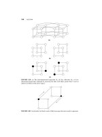
t = 32 illustrates the basic ideas of the Algorithm FGK. The node numbering
for the sibling property is displayed next to each node. The next letter to be processed in the message is
“ai,+, = b". (a) The current status of the dynamic Huffman tree, which is a Huffman tree for 4, the first t letters
in the message.The encoding for “b* is “101 l”, given by the path from the root to the leaf for “b”. (b) The tree
resulting from the interchange process. It is a Huffman tree for 1, and has the property that the weights of the
traversed nodes can be incremented by I without violating the sibling property. (c) The final tree, which is

the tree in (b) with the incrementing done, is a Huffman tree for Ll+, .
FIG. 1. This example from [6] for

Another key concept behind dynamic Huffman codes is the following elegant
so-called characterization of Huffman trees:
Sibling Property: A binary tree with p leaves of nonnegative weight is a
Huffman tree if and only if
(1) the p leaves have nonnegative weights wl, . . . , w,,, and the weight of each
internal node is the sum of the weights of its children; and
(2) the nodes can be numbered in nondecreasing order by weight, so that nodes
2j - 1 and 2j are siblings, for 1 I j 5 p - 1, and their common parent node
is higher in the numbering.
The node numbering corresponds to the order in which the nodes are combined
by Huffman’s algorithm: Nodes 1 and 2 are combined first, nodes 3 and 4 are
combined second, nodes 5 and 6 are combined next, and so on.
Suppose
that ,rU,= ai,, ai2, . . . , ai, has already been processed. The next letter
ai,+, is encoded and decoded using a Huffman tree for Jr. The main difficulty is
how to modify this tree quickly in order to get a Huffman tree for J&+, . Let us
consider the example in Figure 1, for the case t = 32, ai,,, = “b”. It is not good
enough to simply increment by 1 the weights of ai,+,‘sleaf and its ancestors, because


830

JEFFREY SCOTT VITTER

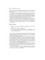
FIG. 2. Algorithm FGK operating on the message “abed . . _“. (a) The
Huffman tree immediately before the fourth letter “d” is processed. The
encoding for “d” is specified by the path to the O-node, namely, “100”. (b) After

Update is called.

the resulting tree will not be a Huffman tree, as it will violate the sibling property.
The nodes will no longer be numbered in nondecreasing order by weight; node 4
will have weight 6, but node 5 will still have weight 5. Such a tree could therefore
not be constructed via Huffman’s two-pass algorithm.
The solution can most easily be described as a two-phase process (although for
implementation purposes both phases can be combined easily into one). In the
first phase, we transform the tree into another Huffman tree for A$, to which
the simple incrementing process described above can be applied successfully in
phase 2 to get a Huffman tree for A$+, . The first phase begins with the leaf of ?,+,
as the current node. We repeatedly interchange the contents of the current node, meluding the subtree rooted there, with that of the highest numbered node of the same
weight, and make the parent of the latter node the new current node. The current
node in Figure la is initially node 2. No interchange is possible, so its parent
(node 4) becomes the new current node. The contents of nodes 4 and 5 are then
interchanged, and node 8 becomes the new current node. Finally, the contents of
nodes 8 and 9 are interchanged, and node 11 becomes the new current node.
The first phase halts when the root is reached. The resulting tree is pictured in
Figure lb. It is easy to verify that it is a Huffman tree for A%~
(i.e., it satisfies the
sibling property), since each interchange operates on nodes of the same weight. In
the second phase, we turn this tree into the desired Huffman tree for &+I by
incrementing the weights of ai,+l’s leaf and its ancestors by 1. Figure lc depicts the
final tree, in which the incrementing is done.
The reason why the final tree is a Huffman tree for A?~+,can be explained in
terms of the sibling property: The numbering of the nodes is the same after the
incrementing as before. Condition 1 and the second part of condition 2 of the
sibling property are trivially preserved by the incrementing. We can thus restrict
our attention to the nodes that are incremented. Before each such node is incremented, it is the largest numbered node of its weight. Hence, its weight can be
increased by 1 without becoming larger than that of the next node in the numbering,

thus preserving the sibling property.
When k < n, we use a single O-node to represent the n - k unused letters in the
alphabet. When the (t + 1)st letter in the messageis processed, if it does not appear
in A& the O-node is split to create a leaf node for it, as illustrated in Figure 2. The


Design and Analysis of Dynamic Huffman Codes

831

(t + 1)st letter is encoded by the path in the tree from the root to the O-node,
followed by some extra bits that specify which of the n - k unused letters it is,
using a simple prefix code.
Phases 1 and 2 can be combined in a single traversal from the leaf of al,+, to the
root, as shown below. Each iteration of the while loop runs in constant time, with
the appropriate data structure, so that the processing time is proportional to the
encoding length. A full implementation appears in [6].
procedure Update;
begin
q := leaf node correspondingto ai,+,;
if (q is the O-node)and (k < n - 1) then
begin
Replaceq by a parent O-nodewith two leaf O-nodechildren, numberedin the order left
child, right child, parent;
q := right child just created
end;

if q is the sibling of a O-nodethen
begin
Interchangeq with the highestnumberedleaf of the sameweight;

Increment q’s weight by 1;
qz; parent of q
;
while q is not the root of the Huffman tree do
begin (Main loop)
Interchangeq with the highestnumberednode of the sameweight:
(q is now the highestnumberednode of its weight)
Increment q’s weight by 1;
q := parent of q
end
end;

We denote an interchange in which q moves up one level by t and an interchange
between q and another node on the same level by +. For example, in Figure 1, the
interchange of nodes 8 and 9 is of type t, whereas that of nodes 4 and 5 is of
type +. Oddly enough, it is also possible for q to move down a level during an
interchange, as illustrated in Figure 3; we denote such an interchange by 4.
No two nodes with the same weight can be more than one level apart in the tree,
except if one is the sibling of the O-node. This follows by contradiction, since
otherwise it will be possible to interchange nodes and get a binary tree having
smaller external weighted path length. Figure 4 shows the result of what would
happen if the letter “c” (rather than “d”) were the next letter processed using the
tree in Figure 2a. The first interchange involves nodes two levels apart; the node
moving up is the sibling of the O-node. We shall designate this type of two-level
interchange by ft. There can be at most one Tt for each call to Update.
3. Analysis of Algorithm FGK
For purposes of comparing the coding efficiency of one-pass Huffman algorithms
with that of the two-pass method, we shall count only the bits corresponding to
the paths traversed in the trees during the coding. For the one-pass algorithms, we
shall not count the bits used to distinguish which new letter is encoded when a

letter is encountered in the messagefor the first time. And, for the two-pass method,
we shall not count the bits required to encode the shape of the tree and the labeling
of the leaves. The noncounted quantity for the one-pass algorithms is typically
between k(log2n - 1) and k logzn bits using a simple prefix code, and the uncounted


832

JEFFREY SCOTT VITTER

(4

(b)
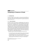
FIG. 3. (a) The Huffman tree formed by Algorithm FGK
after processing “abcdefghiaa”.
(b) The Huffman tree
that will result if the next processed letter is “f “. Note that
there is an interchange of type 4 (between leaf nodes 8 and
10) followed immediately by an interchange of type T
(between internal nodes 11 and 14).

quantity for the two-pass method is roughly 2k bits more than for the one-pass
method. This means that our evaluation of one-pass algorithms will be conservative
with respect to the two-pass method. When the messageis long (that is, t > n),
these uncounted quantities are insignificant compared with the total number of
bits transmitted. (For completeness, the empirical results in Section 5 include
statistics that take into account these extra quantities.)
Definition 3.1. Suppose that a messageMl = ai,, ai,, . . . , ai, of size t 2 0 has
been processed so far. We define St to be the communication cost for a static
Huffman encoding of A& using a Hufman tree based only on A%(;that is,

St = C Wjlj,

where the sum is taken over any Huffman tree for A&. We also define sI to be the
“incremental” cost

s* = s, - Ls,-,.


Design and Analysis of Dynamic Huffman Codes

833

FIG. 4. The Huffman tree that would result from Algorithm FGK if the fourth letter in the example in Figure 2
were “c” rather than “d". An interchange of type TT occurs
when Update is called.

a

We denote by dl the communication cost for encoding ai, using a dynamic Huffman
code; that is,
for the dynamic Huffman tree .with respect to Ml-, . We define D, to be the total
communication cost for all t letters; that is,

D, = D,-, + d,,

Do = 0.

Note that Sodoes not have an intuitive meaning in terms of the length of the
encoding for ai,, as does dt. The following theorem bounds Dl by =2S, + t.
THEOREM 3.1. For each t 2 0, the communication cost of Algorithm FGK can

be bounded by

St - k + 6k=n+ 6k/

I D, 5 2St i- t - 4k + 2&,, i- 26k<, z${Wj)

-

iTI,

I

where & denotes 1 if relation R is true and 0 otherwise, and m is the cardinality of
the set (j 11 I j I t; ail E J&, ; and Qx E dj-1 such that x # a+ x appears strictly
more often in &-, than does ai,).
The term m is the number of times during the course of the algorithm
that the processed leaf is not the O-node and has strictly minimum weight
among all other leaves of positive weight. An immediate lower bound on m is
m 2 min,j,o (Wj) - 1. (For each value 2 5 w 5 min,j,o {Wj), consider the last leaf
to attain weight w.) The minor 6 terms arise because our one-pass algorithms
use a O-node when k < n, as opposed to the conventional two-pass method; this
causes the leaf of minimum positive weight to be one level lower in the tree.
The 6 terms can be effectively ignored when there is a specially designated
“end-of-file” character to denote the end of transmission, because when the
algorithm terminates we have min,+ (Wj1 = 1.
The Fibonacci-like tree in Figure 5 is an example of when the first bound
is tight. The difference Dl - S, decreases by 1 each time a letter not previously
in the messageis processed, except for when k increases from n - 1 to ~1.The
following two examples, in which the communication cost per letter D/t is

bounded by a small constant, yield D/S, + c > 1. The message in the first
example consists of any finite number of letters not including “a” and “b”, followed
by “abbaabbaa
. . .“. In the limit, we have S/t + : and D/t + 2, which
yields D/S, + $ > 1. The second example is a simple modification for the case of


834

JEFFREYSCOTT VITTER

FIG. 5. Illustration of both the lower bound
of Theorem 3.1 and the upper bounds of
Lemma 3.2. The sequence of letters in the messageso far is “abacabdabaceabacabdf” followed by “9” and can be constructed via a simple
Fibonacci-like recurrence. For the lower bound,
let t = 2 1. The tree can be constructed without
any exchanges of types T, tt, or 4; it meets the
first bound given in Theorem 3.1. For the upper
bound, let t = 22. The tree depicts the Huffman
tree immediately before the tth letter is processed. If the tth letter is “h”, we will have
d, = 7 and h, = rd,/21 - 1 = 3. If instead the
tth letter is “g”, we will have d, = 7 and
h, = rd,/21 = 4. If the tth letter is “f”, we will
have d, = 6 and h, = Ld,/2J = 3.

alphabet size n = 3. The messageconsists of the same pattern as above, without
the optional prefix, yielding D,/S, + 2. So far all known examples where
lim sup,,,DJS, # 1 satisfy the constraint D, = 0(t). We conjecture that the
constraint is necessary:

Conjecture. For each t L 0, the communication cost of Algorithm FGK satisfies
D, = S, + O(t).
Before we can prove Theorem 3.1, we must develop the following useful notion.
We shall denote by h, the net change of height in the tree of the leaf for ai, as a
result of interchanges during the tth call to Update.

Definition 3.2. For each t 2 1, we define h, by
h, = (# t’s) + 2(# tt’s) - (# J’s),
where we consider the interchanges that occur during the processing of the tth
letter in the message.
The proof of Theorem 3.1 is based on the following important correspondence
between h, and dt - st:
THEOREM 3.2. For t L 1, we have

4 - St = h, -

aAk=l

+

(6k
T$(Wj),
I

where Af = (f after ai, is processed)- (f before ai, is processed).
PROOF. The 6 terms are due to the presence of the O-node when k < n. Let us
consider the case in which there is no O-node, as in Figure 1. We define 7, to be
the Huffman tree with respect to Al-, , Sb to be the Huffman tree formed by
the interchanges applied to S,, and Z to be the Huffman tree formed from

sb by incrementing a;,‘s leaf and its ancestors. In the example in Figure 1, we
redefine t = 33 and ai, = “b”. The trees S,, sb, and Z correspond to those in
Figure la, lb, and lc, respectively.
Trees S, and sb represent Huffman trees with respect to Ll-, , and Z is a
Huffman tree with respect to Mt. The communication cost dt for processing the tth
letter ai, is the depth in 7, of its leaf node; that is,

d = Ii,(Z)*

(1)


Design and Analysis of Dynamic Hz&man Codes

835

Each interchange of type 7 moves the leaf for ai, one level higher in the tree, each
interchange of type tt moves it two levels higher, and each interchange of type 4
moves it one level lower. We have
h

=

A,(Z)

-

lit(Z).

(2)

The communication costs S,-i and S, are equal to the weighted external path
lengths of S, and Z, respectively. The interchanges that convert 7, to 76 maintain
the sibling property, so S, and sb have the same weighted external path length.
However, yb is special since it can be turned into a Huffman tree for Ml (namely,
tree Z) simply by incrementing ai,‘s leaf and its ancestors by 1. Thus, we have
St = St - St-1 = li,(gb).

(3)

Putting (l), (2), and (3) together yields the result d, - s, = h,.
When there is a O-node present in S,, the communication cost S,-, is
min,c~~~,o(~j(~~)) less than the weighted external path length for S,, since the
presence of the O-node in S, moves a leaf of minimum positive weight one level
farther from the root than it would be if there were no O-node. Similarly, when
there is a O-node in Z, the communication cost S, is min,j(yCj,o {wj(z)) less than
the weighted external path length for Z. If 7, has a O-node and ai, appears in &i,
then the O-node will also appear in Z; this contributes a &<,,A min,+ (wj] term to
d, - s,. If S, has a O-node and at most n - 2 leaves of positive weight, and if ai,
does not appear in J&-~, then the O-node will be split, as outlined in Update; this
has the effect of moving the leaf of ai, one level down, thus contributing
-(dk&,d~k=I) to dl - s,. The final special case is when the O-node appears in S,
but not in Z; in this case, ai, does not appear in A*-, , but the other n - 1 letters
in the alphabet do. This contributes a (~?k=~~~d~k=~)(A
min,>o(wj) - 1) term
to dl - So.Putting these three 6 terms together, with some algebraic manipulation,
gives us the final result. This proves Theorem 3.2. Cl
Three more lemmas are needed for the proof of Theorem 3.1:
LEMMA 3.1. During a call to Update in Algorithm FGK, each interchange of
type 4 is followed at some point by an t, with no J’s in between.

PROOF. By contradiction. Suppose that during a call to Update there are two
interchanges of type 1 with no t in between. In the initial version of the tree before
Update is called, let al and b, be the nodes involved in the first J. interchange
mentioned above, and let a2 and b2 be the nodes in the subsequent J interchange;
nodes al and a2 are one level higher in the tree than bl and b2, respectively, before
Update is called. Let k 2 1 be the number of levels in the tree separating bl and
a2, and let a+ be the ancestor of al that is k levels above al. Node a’; is one level
higher than a2, and we can show that their weights are equal by the following
argument: If the weight of a’; is < al’s weight, then we can interchange the two
nodes and decrease the weighted external path length. On the other hand, if the
weight of a’; is > a2’s weight, then it can be shown from the sibling property that
at some earlier point there should have been an interchange of type 1 in which one
of aI’s ancestors moved down one level. Both cases cause a contradiction. The 5
interchange between a2 and b2 means that b2 has the same weight as a2 and is one
level lower, which makes b2 two levels lower than a: but with the same weight.
This is impossible, as mentioned at the end of Section 2. Cl


836

JEFFREYSCOTTVITTER

LEMMA 3.2. For each t 1 1, we have
Osh,s

I
‘1

rd/2i

- 1,

r4K-n
WY

if ai,‘s node is the O-node;
if ai,‘s node is the O-node’s sibling;
otherwise.

An example achieving each of the three bounds is the Fibonacci-like tree given
in Figure 5.
PROOF. Let us consider what can happen when Update is called to .processthe
tth letter ai,. Suppose for the moment that only interchanges of types t or + occur.
Each t interchange, followed by the statement “q := parent of q”, moves q two
levels up in the tree. A + interchange or no interchange at all, followed by
“q := parent of q”, moves q up one level. Interchanges of type t are not possible
when q is a child of the root. Putting this all together, we find that the
number of T interchanges is at most Ld,/2J, where d* is the initial depth in the tree
of the leaf for ai,.
If there are no interchanges of type Tt or l, the above argument yields
0 I h, 5‘ Ldl/2J. If an interchange of type 1 occurs, then by Lemma 3.1 there is a
subsequent t, so the result still holds. An interchange of type tT can occur if the
leaf for a, is the sibling of the O-node; since at most one TT can occur, we have
0 5 h, 5 rd,/21. The final case to consider occurs when the leaf for af is the O-node;
no interchange can occur during the first trip through the while loop in Update, so
wehaveOsh,(rd,/211. El
LEMMA 3.3. Suppose that ai, occurs in &I, but strictly less often than all the
other letters that appear in A&, . Then when the tth letter in the messageis processed
by Update, the leaffor ai, is not involved in an interchange.
PROOF. By the hypothesis, all the leaves other than the O-node have a strictly

larger weight than ai,‘s leaf. The only node that can have the same weight is its
parent. This happens when ai,‘s leaf is the sibling of the O-node, but there is no
interchange in this special case. Cl
PROOFOF THEOREM3.1. By Lemma 3.2, we have 0 5 h, I dJ2 + i - 6~=, .
Lemma 3.3 says that there are m values oft for which this bound can be lessened
by 1. We get the final result by substituting this into the formula in Theorem 3.2
and by summing on t. This completes the proof. Cl
There are other interesting identities as well, besides the ones given above. For
example, a proof similar to the one for Lemma 3.1 gives the following result:
LEMMA 3.4. In the execution of Update, if an interchange of type t or tt moves
node v upward in the tree, interchanging it with node x, there cannot subsequently
be more T’Sthan J’s until q reaches the lowest common ancestor of v and x.
A slightly weaker bound of the form D, = 2S, + O(t) can be proved using the
following entropy argument suggested by B. Chazelle (personal communication).
The depth of a{s leaf in the dynamic Huffman tree during any of the Wjtimes ai,
is processed can be bounded as a function of the leaf’s relative weight at the time,
which in turn can be bounded in terms of a,‘s final relative weight wJt.
For example, during the last LwG/2J times ail is processed, its relative weight is
rwil/(2t). The factor of 2 in front of the S, term emergesbecause the relative weight
of a leaf node in a Huffman tree can only specify the depth of the node to within
a factor of 2 asymptotically (cf. Lemma 3.2). The characterization we give in


Design and Analysis of Dynamic Hz&man Codes

837

Theorem 3.2 is robust in that it allows us to study precisely how Ot - S, changes
as more letters are processed; this will be crucial for obtaining our main result in
the next section that Algorithm A uses less than one extra bit per letter compared

with the two-pass method.
4. Optimum Dynamic Huffman Codes
In this section we describe Algorithm A and show that it runs in real time and is
optimum in our model of one-passHuffman algorithms. There were two motivating
factors in its design:
(I) The number of t’s should be bounded by some small number (in our case, 1)
during each call to Update.
(2) The dynamic Huffman tree should be constructed to minimize not only
xj Wjlj, but also & 4 and maxi(h), which intuitively has the effect of preventing a lengthy encoding of the next letter in the message.
4.1 IMPLICIT NUMBERING. One of the key ideas of Algorithm A is the use of a
numbering scheme for the nodes that is different from the one used by Algorithm
FGK. We use an implicit numbering, in which the node numbering corresponds
to the visual representation of the tree. That is, the nodes of the tree are numbered
in increasing order by level; nodes on one level are numbered lower than the nodes
on the next higher level. Nodes on the same level are numbered in increasing order
from left to right. We discuss later in this section how to maintain the implicit
numbering via a floating tree data structure.
The node numbering used by Algorithm FGK does not always correspond to
the implicit numbering. For example, the numbering of the nodes in Figures 1, 2,
and 4 does agree with the implicit numbering, whereas the numbering in Figure 3
is quite different. The odd situation in which an interchange of type 4 occurs, such
as in Figure 3, can no longer happen when the implicit numbering is used. The
following lemma lists some useful side effects of implicit numbering.
LEMMA 4.1. With the implicit numbering, interchanges of type 4 cannot occur.
Also, ifthe node that moves up in an interchange of type t is an internal node, then
the node that moves down must be a leaf:

PROOF. The first result is obvious from the definition of implicit numbering.
Suppose that an interchange of type t occurs between two internal nodes a and b,
where a is the node that moves up one level. In the initial tree, since a and b are

on different levels, it follows from the sibling property that both a and b must have
two children each of exactly half their weight. During the previous execution of
the while loop in Update, q is set to a’s right child, which is the highest numbered
node of its weight. But this contradicts the fact that b’s children have the same
weight and are numbered higher in the implicit numbering. Cl
4.2 INVARIANT. The key to minimizing DI - S, is to make t’s impossible,
except for the first iteration of the while loop in Update. We can do that by
maintaining the following invariant:
(*I

For each weight w, all leaves of weight w precede (in the implicit
numbering) all internal nodes of weight w.

Any Huffman tree satisfying (*) also minimizes xjh and maxj(h); this can be
proved using the results of [8]. We shall see later that (*) can be maintained by
floating trees in real time (that is, in O(d,) time for the tth processed letter).


838

JEFFREYSCOTT VI'ITER

LEMMA 4.2. If the invariant (*) is maintained, then interchanges of type tt are
impossible, and the only possible interchanges of type t must involve the moving up
of a leaf:
PROOF. We shall prove both assertions by contradiction. We remarked at the
end of Section 2 that no two nodes of the same weight can be two or more levels
apart in the tree, if we ignore the sibling of the O-node. The effect of the invariant
(a) is to allow consideration of the O-node’s sibling. Let us denote the sibling by p
and its weight by w. Suppose that there is another node p’ of weight w two levels

higher in the tree. By the invariant, node p’ must be an internal node, since it
follows p’s parent (which also has weight w) in the implicit numbering. Each child
of p’ has weight < w, but follows p in the implicit numbering, thus contradicting
the sibling property. For the second assertion, suppose there is an interchange of
type t in which an internal node moves up one level. By Lemma 4.1, the node
that moves down must be a leaf. But this violates the invariant, since the leaf
initially follows the internal node in the implicit numbering. Cl

The main result of the paper is the following theorem. It shows for Algorithm A
that D, - St < t.
THEOREM 4.1.

For Algorithm A, we have

St - k + 6k=n+ 6k1

Wj)

% D, I St i- t - 2k i- (Sk=,,i- &tn

tTZTZ(Wj)
I

-

m.

The 6 terms and the term m 2 min,j,o (Wj) - 1 have the same interpretation as
in Theorem 3.1.

PROOF. By Lemma 4.2, we have 0 I ht 5 6~~0. In addition, there are m values
of t where the upper bound on h, can be decreased from 1 to 0. The theorem
follows by plugging this into the bound in Theorem 3.2 (which holds not only for
Algorithm FGK, but also for Algorithm A) and by summing on t. 0

Remark. It is important to note that the version of Update given in Section 2 is
never executed by Algorithm A. An entirely different Update procedure, which is
given later in this section, is called to maintain invariant (*). But, for purposes of
analysis, a hypothetical execution of the former version of Update does provide,
via Theorem 3.2, a precise characterization of dl - sI.
The lower bound for D, in Theorem 4.1 is the same as in Theorem 3.1, and the
same example shows that it is tight. We can show that the upper bound is tight by
generalizing the D,/S, + 4 and DJS, --j 2 examples in Section 3. For simplicity, let
us assume that n = 2j + 1, for somej L 1. We construct the messagein a “balanced”
“balanced” fashion, so that the weights of n - 1 letters are within 1 of one another,
and the other letter has zero weight. The messagebegins with n - 1 letters in the
alphabet, once each. After .&-i is processed, the leaves of the Huffman tree will
be on the same level, except for two leaves on the next lower level, one of which is
the O-node. At each step, the next letter in the messageis defined inductively to
be the current sibling of the O-node, so as to force dl to be always one more than
the “average” depth of the leaves. We have S, = jt and D, = S, + t - 2n + 3, which
matches the upper bound in Theorem 4.1, since k = n - 1 and m = min,,o( Wj) 1 = Lt/(n - 1)J - 1. Another example consists of appending the nth letter of the
alphabet to the above message.In this case we get St = jt + L(t - l)/(n - I)J + 1
l)J, which again matches the upper
andD,=S+t-2n+2-L(tl)/(nbound, since k = n and m = min,,o(wj) - 1 = L(t - l)/(n - 1)J - 1.


Design and Analysis of Dynamic Huffan

Codes

839

It is important to note that this construction works for any dynamic Huffman
code. The corresponding value of D, will be at least as large as the value of Dt for
Algorithm A. This proves that Algorithm A is optimum in terms of the model we
defined in Section 1:
THEOREM4.2. Algorithm A minimizes the worst-case di&rence
all messages of length t, among all one-pass Huffman algorithms.

D, - S,, over

4.3 OUTLINE OF ALGORITHMA. In order to maintain the invariant (*), we must
keep separate blocks for internal and leaf nodes.
Definition 4.1. Blocks are equivalence classes of nodes defined by v = x iff
nodes v and x have the same weight and are either both internal nodes or both
leaves. The leader of a block is the highest numbered (in the implicit numbering)
node in a block.

The blocks are linked together by increasing order of weight; a leaf block always
precedes an internal block of the same weight. The main operation of the algorithm
needed to maintain invariant (*) is the SlideAndIncrement operation, illustrated in
Figure 6. The version of Update we use for Algorithm A is outlined below:
procedure Update;
begin
leaf ToIncrement := 0;

q := leaf node correspondingto ai,,,;
if (q is the O-node)and (k < n - 1) then
begin 1SpecialCase# 1)

Replaceq by an internal O-nodewith two leaf O-nodechildren, such that the right child
correspondsto at,,,;
q := internal O-nodejust created;
leaf ToIncrement := the right child of q
end
else begin

Interchangeq in the tree with the leaderof its block;
if q is the sibling of the O-nodethen
begin {SpecialCase#2)
leaf ToIncrement := q;
q := parent of q
end
end;
while q is not the root of the Huffman tree do
(Main loop; q must he the leaderof its block]
SlideAndZncrement(q);
if leaf Tolncrement # 0 then (Handle the two specialcases)
SlideAndIncrement(leaf ToIncrement)
end;
procedure SlideAndIncrement(p);
begin
wt := weight of p;
b := block following p’s block in the linked list;
if ((p is a leaf) and (b is the block of internal nodesof weight wt))
or ((p is an internal node) and
(b is the block of leavesof weight wt + 1)) then
begin
Slidep in the tree aheadof the nodesin b;
p’s weight := wt + 1;

if p is a leaf then p := new parent of p
else p := former parent of p
end
end:


840

JEFFREYSCOTT VITTER

(4

04

FIG. 6. Algorithm A’s SIideAndIncrement operation. All the nodes in a given block shift to the left
one spot to make room for node p, which slides over the block to the right. (a) Node p is a leaf of weight
4. The internal nodes of weight 4 shift to the left. (b) Node p is an internal node of weight 8. The leaves
of weight 9 shift to the left.

b

C

(4

a

(b)

FIG. 7. Algorithm A operating on the message“abed . . .“. (a) The Huffman tree immediately before

the fourth letter “d” is processed. (b) After Update is called.

Examples of Algorithm A in operation are given in Figures 7-9; they depict the
same examples used to illustrate Algorithm FGK in Figures 2, 4, and 5. As with
Algorithm FGK, the processing can be done in O(dr+l) time, if the appropriate
data structure is used.
4.4 DATA STRUCTURE. In this section we summarize the main features of our
data structure for Algorithm A. The details and implementation appears in [9].
The main operations that the data structure must support are as follows:
-It

must represent a binary Huffman tree with nonnegative weights that maintains
invariant (*).
-It must store a contiguous list of internal tree nodes in nondecreasing order by
weight; internal nodes of the same weight are ordered with respect to the implicit
numbering. A similar list is stored for the leaves.
-It must find the leader of a node’s block, for any given node, on the basis of the
implicit numbering.
-It must interchange the contents of two leaves of the same weight.


841

Design and Analysis of Dynamic Hufman Codes

FIG. 8. The Huffman tree that would result from
Algorithm A if the fourth letter in the example in
Figure I were “c” rather than “d”.

a

FIG. 9. The Huffman tree constructed by
Algorithm A for the same message used in
Figure 5. Note how much shorter this tree is
compared with the one in Figure 5.

f

e

-It

must increment the weight of the leader of a block by 1, which can cause the
node’s implicit numbering to “slide” past the numberings of the nodes in the
next block, causing their numberings to each decreaseby 1.
-It must represent the correspondence between the k letters of the alphabet that
have appeared in the messageand the positive-weight leaves in the tree.
-It must represent the n-k letters in the alphabet that have not yet appeared in
the messageby a single leaf O-node in the Huffman tree.
The data structure makes use of an explicit numbering, which corresponds to
the physical storage locations used to store information about the nodes. This is
not to be confused with the implicit numbering defined in the last section. Leaf
nodes are explicitly numbered n, n - 1, n - 2, . . . in contiguous locations, and
internal nodes are explicitly numbered 2n - 1, 2n - 2, 212- 3, . . . contiguously;
node q is a leaf iff q I n.
There is a close relationship between the explicit and implicit numberings, as
specified in the second operation listed above: For two internal nodes p and q, we
have p < q in the explicit numbering iff p < q in the implicit numbering; the same
holds for two leaves p and q.
The tree data structure is called a floating tree because the parent and child

pointers for the nodes are not maintained explicitly. Instead, each block has a
parent pointer and a right-child pointer that point to the parent and right child of
the leader of the block. Because of the contiguous storage of leaves and of internal
nodes, the locations of the parents and children of the other nodes in the block can
be computed in constant time via an offset calculation from the block’s parent and
right-child pointer. This allows a node to slide over an entire block without having
to update more than a constant number of pointers. Each execution of SlideAndIncrement thus takes constant time, so the encoding and decoding in Algorithm
A can be done in real time.


842

JEFFREY

SCOTT VI’M’ER

The total amount of storage needed for the data structure is roughly 16n log n +
15n + 2n log t bits, which is about 4n log n bits more than used by the
implementation of Algorithm FGK in [6]. The storage can be reduced slightly by
extra programming. If storage is dynamically allocated, as opposed to preallocated
via arrays, it will typically be much less. The running time is comparable to that
of Algorithm FGK.
One nice feature of a floating tree, due to the use of implicit numbering, is that
the parent of nodes 2j - 1 and 2j is less than the parent of nodes 2j + 1 and
2j + 2 in both the implicit and explicit numberings. Such an invariant is not
maintained by the data structure in [6]; see Figure 3a, for example.

5. Empirical Results
We shall use S,, Dp, and DrGK to denote the communication costs of Huffman’s
algorithm, Algorithm A, and Algorithm FGK. As pointed out at the beginning of

Section 3, our evaluation of one-pass algorithms with respect to Huffman’s twopass method is conservative, since we are granting the two-pass method a handicap
of =2k bits by not including in S, the cost of representing the shape of the Huffman
tree. The costs S,, DF, and D,FGKalso do not count the bits required to encode the
correspondence between the leaves of the tree and the letters of the alphabet that
occur at least once in the message,but this can be expected to be about the same
for the one-pass and two-pass schemes, roughly k(logzn - 1) to k logzn bits using
a simple prefix code.
In this section we report on several experiments comparing the three algorithms
in terms of coding efficiency. The tables below list not only the costs S,, DF, and
DyGK but also the corresponding average number of bits used per letter of the
message(denoted b/l for each of the three methods), which takes into account the
bits needed to describe the tree and the labeling of the leaves. In terms of bits per
letter b/l, Algorithm A actually outperformed the two-pass method in all th’e
experimentsfir which t I 104. Algorithm FGK used slightly more bits per letter,
but also performed well.
Algorithm A has the advantage of using fewer bits per letter for small messages,
where the differences in coding efficiency are relatively more significant. It can be
shown using convergence theorems from statistics that, in the limit as t + 00,the.
communication cost of the one-pass Huffman algorithms is asymptotically equal
to that of the two-pass method for messageswhose letters are generated independently according to some fixed probability distribution (discrete memoryless
source). Even though the messagesused in the longer of our experiments were not
generated in such a manner, they are “sufficiently random” that it is not surprising
that the statistics for the methods are very close for large t.
In the first experiment, the alphabet consisted of the 95 printable ASCII characters, along with the end-of-line character, for a total of n = 96 letters. The
message contained 960 letters: The 96 distinct characters repeated as a group
10 times. This is the type of example where all the methods can be expected to
perform poorly. The static code does the worst. The results are summarized below
at intervals oft = 100, 500, and 96 1:

843

Design and Analysis of Dynamic Hugman Codes

The next example was a variation in which all the methods did very well.
The message consisted of 10 repetitions of the first character of the alphabet,
followed by 10 repetitions of the second character, and so on, for a total message
oft = 960 letters.

~1
The third experiment was performed on the Pascal source code used to obtain
the statistics for St and 0;” reported in this section. Again, alphabet size n = 96 was
t

k

St

b/l

Dt^

b/l

DiGK

v

100
500

1000
10000
12280

34
52
58
74
76

434
2429
-4864
47710
58457

7.1
5.7
5.3
4.8
4.8

420
2445
4900
47852
58614

6.3
5.5

5.2
4.8
4.8

444
2489
4953
47938
58708

6.5
5.6
5.3
4.8
4.8

The fourth experiment was run on the executable code compiled from the Pascal
program mentioned above. The “letters” consisted of 8-bit characters in extended
ASCII, so alphabet size n = 256 was used.
t

k

St

b/l

Dt^

V

Df-

bll

100
500
1000
10000
34817

9
9
9
249
256

124
524
1024
52407
205688

2.1
1.2
1.1
5.5
6.0

117

517
1017
52608
206230

1.9
1.2
1.1
5.4
6.0

122
522
1022
52868
206585

2.0
1.2
1.1
5.5
6.0

The messagefor the final experiment consisted of the device-independent code
for a technical book [lo], written in TPX, with alphabet size n = 256.

I

t

-ijr

100
500
1000
10000
100000
588868

6.7
6.9
7.2
6.9
6.9
7.1

D;=,

378
2625
6029
67997
692858
4171616

6. Conclusions and Open Problems
The proposed Algorithm A performs real-time encoding and decoding of messages
in a single pass, using less than one extra bit per letter to encode the message,as
compared with Huffman’s two-pass algorithm. This is optimum in the worst case,
among all one-pass Huffman methods. The experiments reported in Section 5

indicate that the number of bits used by Algorithm A is roughly equal (and often
better!) than that of the two-pass method. It has much potential for use in file
compression and network communication and for hardware implementation.


844

JEFFREY SCOTT VIl-l'ER

Algorithm FGK performed almost as well in the experiments. We conjecture
that Algorithm FGK uses 0( 1) extra bits per letter over the two-pass method in
the worst case. Note that this does not contradict the examples that appear after
Theorem 3.1, for which D,/St > 1, since in each case the communication cost per
letter is bounded, that is, D, = 0(t). Figure 5 shows that dt # So+ O(l), so a proof
of the conjecture would require an amortized approach.
The one-pass Huffman algorithms we discuss in this paper can be generalized to
d-way trees, for d L 2, for the case in which base-d digits are transmitted instead
of bits. Algorithm A can also be modified to support the use of a “window” of size
b > 0, as in [6]. Whenever the next letter in the messageis processed, its weight in
the tree is increased by 1, and the weight of the letter processed b letters ago is
decreasedby 1. This technique would work well for the second experiment reported
in the previous section.
Huffman coding does not have to be done letter by letter. An alternative well
suited for tile compression in some domains is to break up the message into
maximal-length alphanumeric words and nonalphanumeric words. Each such word
is treated as a single “letter” of the alphabet. One Huffman tree can be used for the
alphanumeric words, and another for the nonalphanumeric words. The final sizes
of the Huffman trees are proportional to the number of distinct words used. In
many computer programs written in a high-level language, for example, the
vocabulary consists of some variable names and a few frequently used keywords,

such as “while”, “*off”, and “end”, so the alphabet size is reasonable. The alphabet
size must be bounded beforehand in order for one-pass Huffman algorithms to
work efftciently.
Algorithm A can also be used to enhance other compression schemes, such as
the one-pass method described and analyzed in [ 11, which is typically used in a
word-based setting. A self-organizing cache of size c is used to store representatives
of the last c distinct words encountered in the message.When the next word in the
messageis processed, let 1,where 1 I 1I c, denote its current position in the cache;
if the word is not in the cache, we define I= c + 1. The word is encoded by an
encoding of 1, using a suitable prefix code. If 1 = c + 1, this is followed by the
encoding of the individual letters in the word, using a separate prefix code. The
word’s representative is then moved to the front of the cache, bumping other
representatives down by one if necessary, and the next word in the message is
processed. Similar algorithms are also considered in [2]. The algorithm can be
made to run in real time by use of balanced tree techniques, and it uses no more
than St + t + 2t log( 1 + SJt) bits to encode a message containing t words, not
counting the extra bits required when the representative is not in the cache. (It is
interesting to compare this bound with the corresponding bound S, + t - 1 for
Algorithm A, which follows from Theorem 4.1.) For any given word that appears
more than once in the message,its representative can potentially be absent from
the cache each time it is processed,and whenever it is absent, extra bits are required.
The method achieves its best coding efficiency when the two prefix codes (used to
encode 1 and the letters in the words for which I= c + 1) are dynamic Huffman
codes constructed by Algorithm A.
ACKNOWLEDGMENTS.
The author would like to thank Marc Brown, Bernard
Chazelle, and Bob Sedgewick for interesting discussions. Marc’s animated
Macintosh implementation of Algorithm FGK helped greatly in the testing
of Algorithm A and in the preparation of the figures. The entropy argument

Design and Analysis of Dynamic Hugman Codes

845

mentioned at the end of Section 3 is due to Bernard. Bob suggested the
D,/S, + $ example in Section 3. Thanks also go to the referees for their very
helpful comments.
REFERENCES
I. BENTLEY, J. L., SLEATOR,D. D., TARJAN, R. E., AND WEI, V. K. A locally adaptive data
compression scheme. Commun. ACM 29,4 (Apr. 1986), 320-330.
2. ELIAS,P. Interval and recency-rank source coding: Two online adaptive variable-length schemes.
IEEE Trans. InJ Theory. To be published.
3. FALLER,N. An adaptive system for data compression. In Record ofthe 7th Asilomar Conference
on Circuits, Systems, and Computers. 1913, pp. 593-591.
4. GALLAGER,R. G. Variations on a theme by Huffman. IEEE Trans. Inj Theory IT-24, 6 (Nov.
1978), 668-674.
5. HUFFMAN,D. A. A method for the construction of minimum redundancy codes. In Proc. IRE 40
(1951), 1098-1101.
6. KNUTH, D. E. Dynamic Huffman coding. J. Algorithms 6 (1985), 163-180.
7. MCMASTER, C. L. Documentation of the compact command. In UNIX User’s Manual, 4.2
Berkeley Software Distribution, Virtual VAX- I I Version, Univ. of California, Berkeley, Berkeley,
,
Calif., Mar. 1984.
8. SCHWARTZ,E. S. An Optimum Encoding with Minimum Longest Code and Total Number of
Digits. If: Control 7, 1 (Mar. 1964), 37-44.
9. VIITER, J. S. Dynamic Huffman Coding. ACM Trans. Math. Sojlw. Submitted 1986.
10. VIITER, J. S., AND CHEN, W. C. Design and Analysis of Coalesced Hashing. Oxford University
Press,New York, 1987.
RECEIvEDJUNE 1985; REVISEDJANUARY1987; ACCEPTEDAPRIL 1987

JournaloftheAsociationforComputing
Machioery,
Vol.34,No.4,baobcr 1987.