Multichannel communication based on adaptive equalization in very shallow water acoustic channels
Bạn đang xem bản rút gọn của tài liệu. Xem và tải ngay bản đầy đủ của tài liệu tại đây (1.82 MB, 100 trang )
MULTICHANNEL COMMUNICATION BASED ON
ADAPTIVE EQUALIZATION IN VERY SHALLOW
WATER ACOUSTIC CHANNELS
TAN BIEN AIK
(B.Eng. (Hons.), NUS)
A THESIS SUBMITTED
FOR THE DEGREE OF MASTER OF ENGINEERING
DEPARTMENT OF ELECTRICAL AND COMPUTER
ENGINEERING
NATIONAL UNIVERSITY OF SINGAPORE
ACKNOWLEDGEMENTS
The author would like to thank his supervisors, Dr Mehul Motani, who is an
Assistant Professor in Electrical and Computer Engineering department at the National
University of Singapore, Associate Professor John R. Potter, who is an Associate
Director of Tropical Marine Science Institute at the National University of Singapore
and Dr. Mandar A. Chitre, who is the Deputy Head of Acoustic Research Laboratory
at the National University of Singapore, for their time and invaluable guidance
throughout the progress of this thesis.
The author wishes to thank DSO National Laboratories for making the data
available. The author would also like to thank his DSO colleagues
Mr Koh Tiong
Aik, Mr Quek Swee Sen and Mr Zhong Kun for their help with the sea trial
experiments and data transmissions/acquisitions and in addition, Mr Quek Swee Sen
again for the help and contributions for the turbo product code notes and MATLAB®
functions that were provided for in this thesis.
This thesis will not be possible without the understanding and support from the
author s family and Miss Nina Chun.
Page-i
TABLE OF CONTENTS
Acknowledgements
i
Summary
iv
List of Tables
v
List of Figures
vii
List of Symbols and Abbreviations
x
Chapter 1 Introduction ................................................................................................1
1.1
1.2
1.3
Literature Review ....................................................................................1
Contributions ...........................................................................................6
Thesis Outline..........................................................................................7
Chapter 2 Underwater Acoustic Channel ..................................................................8
2.1
2.1.1
2.1.2
2.1.3
2.1.4
2.1.5
2.1.6
2.1.7
2.2
2.2.1
2.2.2
Propagation Model ..................................................................................8
Sound Velocity ......................................................................................12
Spreading Loss ......................................................................................13
Attenuation Loss....................................................................................13
Surface Reflection Loss.........................................................................15
Bottom Reflection Loss .........................................................................15
Combined Received Response ..............................................................16
Time Varying Channel Response ..........................................................17
Channel Measurements..........................................................................18
Experimental Setup................................................................................18
Multipath Power Delay Profile, Delay Spread and Coherence
Bandwidth..............................................................................................18
2.2.2.1 Delay Spread .....................................................................................23
2.2.2.2 Coherence Bandwidth .......................................................................24
2.2.3
Doppler Effects......................................................................................26
2.2.3.1 Doppler Spread..................................................................................30
2.2.3.2 Coherence TIme ................................................................................31
2.2.4
Ambient Noise.......................................................................................35
2.2.4.1 Stable and Gaussian Distributions.....................................................35
2.2.4.2 Amplitude Distribution Results.........................................................36
2.2.4.3 Noise Spectrum .................................................................................37
2.2.4.4 Range, Bandwidth and Signal to Noise Ratio (SNR)........................39
2.2.5
Signal Envelope Fading Characteristics ................................................41
Chapter 3 Preliminary DPSK Performance in Channel Simulator and Sea Trial ..
...........................................................................................................46
3.1
3.2
Channel Simulator .................................................................................46
Sea Trial.................................................................................................48
Page-ii
Chapter 4 Adaptive equalization, Multichannel Combining and Channel Coding .
...........................................................................................................51
4.1
4.2
4.3
4.4
4.5
4.6
4.7
4.8
4.9
4.10
Linear and Decision Feedback Equalizers.............................................51
LE-LMS Performance in Simulation.....................................................59
LE-LMS Performance in Sea Trial........................................................60
DFE-LMS Performance in Sea Trial .....................................................63
A Note on Sparse DFE-LMS Performance in Sea Trial........................64
LE-RLS Performance in Sea Trial.........................................................66
DFE-RLS Performance in Sea Trial ......................................................67
Performance Comparison for DFE, LE, LMS and RLS........................68
Multichannel Combining.......................................................................69
Channel Coding .....................................................................................75
Chapter 5 Conclusion.................................................................................................79
Chapter 6 Future Work .............................................................................................80
Bibliography
...........................................................................................................81
Page-iii
SUMMARY
Very shallow water acoustic communication channels are known to exhibit
fading due to time-varying multipath arrivals. This is further complicated by impulsive
snapping shrimp noise that is commonly present in warm shallow waters. Channel
measurements and analyses were done to study the local shallow water characteristics.
These measurements had helped verify and set the communication channel model and
adaptive receivers presented in this thesis. This thesis also presents results from the use
of single-carrier differential phase shift keying (DPSK) modulation. The receiver
designs in the simulation and trial data analysis were based on combinations of least
mean square (LMS) and recursive least square (RLS) algorithms with adaptive linear
equalizer (LE) and decision feedback equalizer (DFE). In addition, multichannel
combining (MC) and forward error correction (FEC) scheme such as turbo product
codes (TPC) were employed to improve performance by removing correctable errors.
Performance results based on simulated data as well as for real data collected from the
sea were also presented.
Page-iv
LIST OF TABLES
Table 2-1.
Applicability of propagation models [3]....................................................9
Table 2-2.
Sea trial parameters..................................................................................19
Table 2-3.
Delay spread and coherence bandwidth results for different ranges .......25
Table 2-4.
Doppler and coherence time results for different ranges .........................34
Table 2-5.
Overall results for signal envelope fading for different ranges ...............44
Table 3-1.
Simulation parameters..............................................................................47
Table 3-2
Simulated BER results of binary DPSK in shallow water channels ........48
Table 3-3.
Delay spread and coherence bandwidth results for different ranges .......50
Table 3-4.
Trial BER results of DBPSK in shallow water channels
Table 4-1.
Summary of LE-LMS algorithm..............................................................55
Table 4-2.
Summary of DFE-LMS algorithm ...........................................................56
Table 4-3.
Summary of LE-RLS algorithm...............................................................57
Table 4-4.
Summary of DFE-RLS algorithm ............................................................58
Table 4-5.
Simulated BER results of DBPSK in shallow water channels after LELMS .........................................................................................................59
Table 4-6.
Trial BER results of DBPSK in shallow water channels after LE LMS,
Channel one..............................................................................................61
Table 4-7.
Trial BER results of DBPSK in shallow water channels after DFE LMS,
Channel one..............................................................................................63
Table 4-8
Trial BER results of DBPSK in shallow water channels after Sparse
DFE LMS, Channel one..........................................................................65
Table 4-9.
Trial BER results of DBPSK in shallow water channels after LE RLS,
Channel one..............................................................................................66
Channel one.50
Table 4-10. Trial BER results of DBPSK in shallow water channels after DFE RLS,
Channel one..............................................................................................68
Table 4-11. Trial BER Results of DBPSK in Shallow Water Channels after LE-LMS
and MC.....................................................................................................73
Table 4-12. Trial BER Results of DBPSK in Shallow Water Channels after LE-RLS
and MC.....................................................................................................74
Page-v
Table 4-13. Trial BER Results of DBPSK in Shallow Water Channels after LE-LMS,
MC and TPC ............................................................................................77
Table 4-14. Trial BER Results of DBPSK in Shallow Water Channels after LE-RLS,
MC and TPC ............................................................................................77
Page-vi
LIST OF FIGURES
Figure 2-1. Methods to solve the Helmholtz equation .................................................9
Figure 2-2. Shallow water multipath model from [10]...............................................10
Figure 2-3. Typical sound velocity profile in local waters .........................................12
Figure 2-4. Volume attenuation for sea water at temperature of 29 c given by the
Hall-Watson formula................................................................................14
Figure 2-5. Sea trial setup ...........................................................................................19
Figure 2-6. Simulated channel impulse response for 80m and 2740m respectively ..20
Figure 2-7. Multipath delay profiles with time shifts due to ships motion. ..............21
Figure 2-8. Multipath delay profiles after MSE alignment. .......................................21
Figure 2-9. Average multipath power delay profile ...................................................21
Figure 2-10. Channel impulse response - MPDPs close up plot for first five seconds 22
Figure 2-11. Average multipath power delay profiles (Top:80m, Bottom:2740m) after
flooring at 20dB .......................................................................................24
Figure 2-12. Multi-Doppler matched filter after demodulation [38] ............................27
Figure 2-13. Doppler resolution/ambiguity functions of various length BPSK msequence ...................................................................................................29
Figure 2-14. Typical Doppler spectrum........................................................................31
Figure 2-15. Spaced time correlation function .............................................................32
Figure 2-16. Delay Doppler measurements of BPSK m-sequence 80m.......................33
Figure 2-17 Doppler spectrum of BPSK m-sequence 80m .........................................33
Figure 2-18. Delay Doppler measurements of BPSK m-sequence 2740m...................33
Figure 2-19. Doppler spectrum of BPSK m-Sequence 2740m.....................................34
Figure 2-20. Comparison of various histograms versus measured ambient noise
histogram..................................................................................................36
Figure 2-21. Ambient noise spectrum...........................................................................38
Figure 2-22. Amplitude waveform of ambient noise showing its impulsive nature (of
snapping shrimp origin) ...........................................................................38
Figure 2-23. SNR performance over distance and centre frequency............................40
Page-vii
Figure 2-24. SNR performance over frequency at 4km................................................40
Figure 2-25. Comparative and measured PDFs for signal envelope received at 80m..43
Figure 2-26. Comparative and measured CDFs for signal envelope received at 80m. 43
Figure 2-27. Comparative and measured PDFs for signal envelope received at 2740m
..................................................................................................................44
Figure 2-28. Comparative and measured PDFs for signal envelope received at 2740m
..................................................................................................................44
Figure 3-1. Multipath profile measurement from sea trial (80m)...............................46
Figure 3-2. Multipath profile of channel simulator (80m)..........................................46
Figure 3-3. DBPSK frame format...............................................................................47
Figure 3-4. Comparing BERs of trial and simulated data for the same distance........50
Figure 4-1. Linear equalizer........................................................................................51
Figure 4-2. Decision feedback equalizer ....................................................................52
Figure 4-3. Simulated LE-LMS equalization-distance: 1040m (a) Mean square error
(b) Filter tap coefficients (c)Input I-Q plot of differential decoded r(k) (d)
Output I-Q plot of a (k ) ...........................................................................60
Figure 4-4
Comparing BERs of trial and simulated data for the same distance after
equalization ..............................................................................................61
Figure 4-5. LE-LMS equalization on trial data-distance: 1040m (a) Mean square error
(b) Filter tap coefficients (c) Input I-Q plot of differential decoded r(k)
(d) Output I-Q plot of a(k ) .....................................................................62
Figure 4-6
Comparing DFE-LMS and sparse DFE-LMS performance ....................65
Figure 4-7. LE-RLS equalization on trial data-distance: 1040m (a) Mean square error
(b) Filter tap coefficients (c) Input I-Q plot of differential decoded r(k)
(d) Output I-Q plot of a(k ) .....................................................................67
Figure 4-8
BER performance of Equalizers: LE-LMS, DFE-LMS, LE-RLS and
DFE-RLS .................................................................................................69
Figure 4-9. Multichannel combining method with LE or DFE ..................................70
Figure 4-10. Multichannel combining with LE-LMS equalization-distance: 2740m (a)
Mean square error (b) Filter tap coefficients (c)Input I-Q plot of
differential decoded r(k) (d) single channel output I-Q plot of a (k ) (e)
Multiple channel combined IQ Plot .........................................................71
Figure 4-11 BER performances of multichannel combining.......................................72
Page-viii
Figure 4-12 Percentage of error free frames after multichannel combining................72
Figure 4-13. Turbo product code (TPC) encoder structure ..........................................75
Figure 4-14 BER performances of different schemes .................................................78
Figure 4-15. Error-free frame performances of different schemes ...............................78
Page-ix
LIST OF SYMBOLS AND ABBREVIATIONS
Symbols
L
Horizontal distance between the transmitter and receiver
t
Continuous time index
a
Depth of transmitter
b
Depth of receiver
A
A coefficient associated with the Lyords mirror effects
h
Bottom depth
D
Distance traveled by direct ray in Ray Theory
n
Order of reflections
SSn
nth signal path, in distance, which makes the first and last boundary reflection
with the surface
SBn
nth signal path, in distance, which makes the first boundary reflection with the
surface and last boundary reflection with the bottom
BSn
nth signal path, in distance, which makes the first boundary reflection with the
bottom and last boundary reflection with the surface
BBn
nth signal path, in distance, which makes the first and last boundary reflection
with the bottom
c
Underwater sound velocity
tD
Arrival time of direct arrival
tSSn
Arrival time of SSn
tSBn
Arrival time of SBn
t BSn
Arrival time of BSn
t BBn
Arrival time of BBn
SSn
Propagation delay of SSn relative to the direct arrival
SBn
Propagation delay of SBn relative to the direct arrival
BSn
Propagation delay of BSn relative to the direct arrival
Page-x
BBn
kc
Propagation delay of BBn relative to the direct arrival
A coefficient associated with the angle of arrival of the acoustic ray at the
receiver
Angle of arrival of the acoustic ray at the receiver
Ls
dB / km
Spreading loss of an omni-directional acoustic pressure wave
Frequency dependent attenuation loss in decibels per kilometre
LA
Attenuation factor
f
Acoustic frequency in kHz
fc
Acoustic carrier frequency in kHz
fT
A coefficient associated with the frequency dependent attenuation loss
Tw
Temperature of water in degrees Fahrenheit
TdegC
Temperature of water in degrees Celsius
rs
Surface reflection loss
rb
Bottom reflection loss
f1
A coefficient associated with the surface reflection loss
f2
A coefficient associated with the surface reflection loss
Density
m
Ratio of bottom density to water density
nc
Ratio of sound velocity in water to sound velocity in bottom
Grazing angle of the incident acoustic ray with the bottom
RSSn
Combined reflection loss of a nth order SS acoustic ray
RSBn
Combined reflection loss of a nth order SB acoustic ray
RBSn
Combined reflection loss of a nth order BS acoustic ray
RBBn
Combined reflection loss of a nth order BB acoustic ray
x(t)
Transmitted Signal
Page-xi
r(t)
Received Signal
Combined transmission loss of the acoustic ray
P
Average power delay profile
Ei
ith Power delay profile
h( )
Bandpass impulse response
Tm
Excessive delay spread
Root mean squared delay spread
Ts
Symbol period
Bc
Coherence bandwidth
fd
Doppler spread
To
Coherence time
S(v)
Scattering function
S(f)
Doppler spectrum
t Space time correlation function
k
Discrete time index
a(k)
Original bit sequence
d(k)
Differentially encoded bit sequence
z(k)
Differentially decoded soft output sequence
r(k)
Complex baseband received signal
a(k )
Estimated original bit sequence
e(k)
Error signal
y(k)
Adaptive filter output
r(2k) Adaptive filter input vector
b(k)
Training Signal/Tracking Signal
ff(k)
Feed forward fitler tap coefficient vector
ff
Feed forward adaptation step size
Page-xii
N
Number of filter taps
Nf
Number of feed forward filter taps
Nb
Number of feed back filter taps
fb
Feed back tap adaptation step size
b(k)
Feed back vector
fb(k)
Feed back fitler tap coefficient vector
A coefficient associated with RLS algorithm
Forgetting factor of the RLS algorithm
1
A Nf + Nb square matrix of the RLS algorithm
ku
A coefficient associated with the TPC encoder structure
nd
A coefficient associated with the TPC encoder structure
ce(k)
Channel effects sequence
dc(k)
Differentially encoded TPC codeword
ac(k)
TPC Codeword
yc(k)
Adaptive filter output of differentially encoded TPC codeword
Phase offset of adaptive filter output
n(k)
Noise signal component of adaptive filter output
Page-xiii
Abbreviations
BER
Bit Error Rate
BPSK
Binary Phase Shift Keying
DBPSK
Differential Binary Phase Shift Keying
CDF
Cumulative Distribution Funtion
CW
Continuous Wave
DFE
Decision Feedback Equalizer
DPSK
Differential Phase Shift Keying
FIR
Finite Impulse Response
FER
Frame Error Rate
GPS
Global Positioning System
IIR
Infinite Impulse Response
ISI
Inter Symbol Interference
LE
Linear Equalizer
LMS
Least Mean Square
LOS
Line Of Sight
MC
Multichannel Combining
MIMO
Multiple Input Multiple Output
MPDP
Multipath Power Delay Profile
MMSE
Minimum Mean Square Error
MSE
Mean Square Error
OFDM
Orthogonal Frequency Division Multiplexing
PAPR
Peak to Average Power Ratio
PC
Personal Computer
Probability Density Function
PN
Pseudo Noise
RLS
Recursive Least Square
Page-xiv
RMS
Root Mean Square
SISO
Soft-Input-Soft-Output
SNR
Signal to Noise Ratio
TPC
Turbo Product Code
Page-xv
CHAPTER 1 INTRODUCTION
1.1
Literature Review
The recorded history of underwater acoustics dates back to 1490 when
Leonardo da Vinci wrote [1]: If you cause your ship to stop, and place the head of a
long tube in the water and place the outer extremity to your ear, you will hear ships at
a great distance from you.
This remarkable disclosure has helped to develop many
modern underwater acoustic technologies for civil and military applications. These
include fishing, submarine, bathymetric and side scan SONARs, echo sounders,
Doppler velocity loggers, acoustic positioning systems, and more importantly,
underwater acoustic communications system, which is of considerable interest in
today s research. The technological advent of underwater explorations and sensing
applications such as unmanned/autonomous underwater vehicles (U/AUVs), offshore
oil and gas operations, ocean bottom monitoring stations, remote mine hunting and
underwater structure inspections have driven the need for underwater wireless
communications. Sound transmission is the single most effective means of directing
energy transfer over long distances in sea-water. Radio-wave propagation is ineffective
for this purpose because all but the lowest usable frequencies attenuates rapidly in the
conducting sea water. And, optical propagation is subjected to scattering by suspended
material in the sea [2, pp. 1.1-1.2].
What do we know about the shallow acoustic communication channel and how
do we characterize it? Very shallow water acoustic communication channel
is
generally characterized as a multipath channel due to the acoustic signal reflections
from the surface and the bottom of the sea [3]. However, it is also well known that the
shallow water channel exhibits time varying multipath fading [4-6]. Time variability
in the channel response results from a few underwater phenomena. Random signal
fluctuation due to micro-paths [7] is one of the phenomenon but it is more dominant in
Page-1
deep oceans where there are stronger presence of internal waves and turbulence [8].
For shallow waters, micro-paths of each signal path are less dominant in contributing
to random signal fluctuation and these micro-paths are generated from the acoustic
scattering caused by small inhomogeneities in the medium and other suspended
scatterers. In addition, surface scattering due to surface waves and random Doppler
spreading of surface reflected signals due to motion of reflection point may have added
to the channel s time variability for shallow water [4]. As a result, the signal multipath
components undergo time-varying propagation delays, resulting in signal fading. This
is further complicated by impulsive snapping shrimp noise that is commonly present in
Singapore's warm waters [6, 9]. Propagation in shallow water may be modeled using
Ray theory, Normal mode, Fast Field or Parabolic Equation method [3, p. 223]. For
high frequencies in shallow water, Ray theory is one such model that is adequate to
describe the multipath structure of the channel [3]. Zielinksi [10] presented a simple
and practical time invariant shallow water ray model for acoustic communications.
Yeo [11] extended Zielinski s work and verified experimentally that the model is
appropriate for shallow water channels. Later, Geng and Zielinski [12] also claimed
that the underwater channel is not a fully scattering channel where there may be
several distinct eigenpaths linking the transmitter and receiver. Each distinct eigenpath
may contain a dominant component and a number of random sub-eigenpath
components. Recently, Gutierrez [13] also proposed an eigenpath model with random
sub-eigenpath components. As there were a lack of sea experimental analysis to verify
the models from [12, 13], this thesis adopted the model in [10]. As for time variability,
Chitre [6, 14] had proposed using Rayleigh fading model with some local sea trial data
analyses backing (very short distances < 100m). This is similar to the Rayleigh fading
model that is commonly used in radio communications [15, pp. 222-223]. The model
Page-2
presented in this thesis is based on [10] and its time variability effect is based on [6,
14, 15].
One of the earliest underwater communication systems was a submarine s
underwater telephone developed by the United States in 1945 [16]. It can be used for
several kilometres and employed single side band modulation in the band of 8-11kHz.
In recent years, significant advancements have been made in the development of
underwater acoustic digital communications with improved communication distance
and data throughput [4, 5]. The main performance limitations of the underwater
acoustic communications are channel phase stability, available bandwidth and channel
impulse response fluctuation rate [5]. To overcome these difficulties, the design of
commercially available underwater modems has mostly relied on the use of robust
non-coherent and spread spectrum modulation techniques. Unfortunately, these
techniques were known to be bandwidth inefficient and it will be difficult to achieve
high data rates in the severely band limited underwater acoustic channel ~ typically,
less than 1 kilobits per second (kbps) or about 0.02 to 0.2 bits/Hz efficiency for
distances between one to two kilometers (according to some COTS underwater modem
specifications). Some of these commercial modems had been deployed in our local,
very shallow waters of depths of less than 30m with impulsive noise. These modems,
that had worked well in other channels, performed poorly by having to set its baud rate
to the lowest in order to achieve reliable communications (~100-300bps) for distances
up to 2km. On the other hand, research focus had shifted to phase-coherent modulation
techniques. The most noticeable was the coherent detection of digital signals at 3040kbps for a time varying 1.8km shallow water channel presented by Stojanovic [4] in
1997. These advanced techniques have yet to be used in commercially available
acoustic modems.
Page-3
Recently, channel measurements at medium frequency ranges (9-28kHz) in
very shallow water (15-30m) at distances ranging from 80m to 2.7km in the coastal sea
of Singapore have shown that it is possible to reliably send high data rate
communication signals [17]. It also highlighted that it is more difficult to obtain the
same high data rates (that is achievable at longer distances1) at shorter distances due to
increased delay and Doppler spreads. These were supported by some local
development work on orthogonal frequency division multiplexing (OFDM) by [14, 18,
19].
OFDM has been successful in achieving higher data rates in multipath
environment without the help of channel equalization as it avoid inter symbol
interference (ISI) effects by sending multiple low rate sub-carrier signals
simultaneously with time guards called cyclic prefix and postfix. In [19], the OFDM
modem had a maximum data rate of 10kbps at 1700m but it had to step down its data
rates as the distance reduces. This is because using OFDM alone (without
equalization) to combat the multipath effect often force system designers to reduce
data rate in more severe time-dispersive channels.
The increase in delay spread
effectively increases the time guards required. Despite this, their frequency diversity or
multi-carrier modulation techniques have produced reliable and higher data rates when
compared to some of the COTS modems available. However, OFDM do have some
drawbacks. High peak to average power ratio (PAPR) in OFDM transmission is
inherent and it will need special coding scheme to reduce the PAPR. OFDM also have
training/tracking problems in adaptive equalization of its low rate sub-carrier signals if
it wants to maintain high bit rates for a wider range of delay spreads. Finally, in mobile
underwater communications, a more complicated Doppler correction algorithm for the
multi-carrier system is needed when compared to one in a single carrier system. Some
1
As the bottom depth for the sea trial experiments and simulation does not vary much (~15m to 30m),
long distances mentioned here usually meant that the range depth ratio is large (larger than 30).
Page-4
other possible techniques/enablers for high data rate are single carrier modulation with
adaptive equalization [8, 20-22], adaptive multichannel combining [20, 23-25] and
multiple input multiple output (MIMO) / Time Reversal (TR) system [26-28]. MIMO
system leverages on space-time diversity to increase data rate. In a MIMO wireless
link, the data stream is broken into separate signals and sent through separable
multipath channels in space. In underwater, MIMO system, such as in [26, 27], may
require the projector and receiver arrays to span across a few meters or even the water
column in order to exploit the multipath channel. This will result in making the MIMO
system setup too bulky. While adaptive equalization and multichannel combining has
not been explored in our local waters, they do not suffer the drawbacks of OFDM and
still remain physically compact unlike MIMO. The disadvantage of single carrier multichannel communication with adaptive equalization is the higher order of
complexity of implementation when compared to multi-carrier - OFDM alone.
Therefore this thesis will experiment the sea data with single carrier adaptive
equalization and multichannel combining to provide consistent high and reliable data
rate over the challenging channels described above. Single carrier DPSK was chosen
as it does not require an elaborate method for estimating the carrier phase.
Apart from using MIMO to exploit the multipath structure of the underwater
channel, can we exploit some other knowledge about the channel in communication
signal processing? Channel measurements in [17] had shown that the shallow water
multipath power delay profiles were sparse and these were prevalent in short distances.
Some proposed exploits in sparse multipath channels were found in [29, 30]. The
length of adaptive equalizer in underwater communications was known to be
excessively long due to long delay spreads. This poses three problems: an increase in
computational complexity, slower convergence rate and the increased noise in channel
Page-5
equalization. In Kocic [29], the aim of the work was to reduce the complexity of the
adaptive equalizer by exploiting the sparse multipath channel. As the threshold to deactivate taps in [29] was considered high, the effect would be a significant reduction in
computational load with negligible loss in performance.
Similarly, having large
number of filter taps also slows down the convergence process of the equalizer as the
step size has to be reduced to guarantee stability. To address the slow convergence
problem in fast fading and long delay channels, Heo [30] proposed channel estimate
based tap initialization and sparse equalization to hasten the convergence process. This
result in faster initial and nominal convergence and a one-two decibel increase in
signal to noise ratio (SNR), when compared to the conventional approach. This thesis
will explore sparse equalization to reduce noise in the estimate of inverse channel so as
to improve the BER performance of the equalizer.
1.2
Contributions
Channel measurements and analyses were done to study the local shallow
water characteristics. These measurements had helped verify the communication
channel model presented in this thesis.
The reader may also find the channel
measurement sections useful in designing communication system. This thesis had
presented results from the use of single-carrier differential phase shift keying (DPSK)
modulation. The receiver designs in sea trial data analyses were based on combinations
of least mean square (LMS) and recursive least square (RLS) algorithms with adaptive
linear equalizer (LE) and decision feedback equalizer (DFE). The LE-LMS receiver
was simulated using the channel model simulator for all distances tested and the
simulated results were approximately matched to the ones obtained from the sea trial.
In order to achieve reliable communications, multichannel combining (MC) and
forward error correction (FEC) scheme such as turbo product codes (TPC) were
Page-6
employed to improve performance by removing correctable errors. These results a
detailed performance analyses of different equalizers and adaptation algorithms over a
range of communication distances (80m to 2740m). In addition, sparse equalization
had been explored in order to exploit the sparse channel and reduce the noise in the
inverse channel estimate of adaptive equalizers. Performance results were based on
real data collected from the sea.
1.3
Thesis Outline
The thesis is organised into four main chapters. The first chapter presents the
literature review. The first half of chapter two presents a propagation channel model
that is suitable for our shallow water geophysics. Remaining parts of the second
chapter attempts to characterize underwater communication channel as well as to
obtain the parameters for channel model simulations and adaptive receivers. Chapter
three verifies the channel simulator, discussed in chapter one and two, by digital
communication performance analysis via simulation as well as sea trial data. Finally,
in chapter four, sea trial and some simulated performance of adaptive equalization
algorithms, sparse equalization, multichannel combining and channel coding were
presented.
Page-7
CHAPTER 2 UNDERWATER ACOUSTIC CHANNEL
An underwater acoustic channel is characterized as a multipath channel due to
signal reflections from the surface and the bottom of the sea. Because of surface wave
motion, the signal multipath components undergo time varying propagation delays that
results in signal fading. In addition, there is frequency dependent attenuation which is
approximately proportional to the square of the signal frequency. The sound velocity is
nominally about 1540m/s but the actual value will vary either above or below the
nominal value depending on the temperature, salinity and hydrostatic pressure at which
the signal propagates. Ambient ocean acoustic noise is caused by shrimp, fish, and
various mammals. Unfortunately, ocean ambient noise also includes man made
acoustic noise such as seismic surveys, ship traffic and land reclamation. When sound
propagates underwater, it undergoes a number of effects. The following sections will
briefly explain these effects.
2.1
Propagation Model
There are many methods of multipath modeling. Figure 2.1 shows the general
techniques used [3] to solve the Helmholtz (Wave) equation in acoustic propagation
modeling. For shallow water channel, the acoustic characteristics of both the surface
and bottom of the channel are important determinants of the sound field due to
repeated reflections from both the surface and bottom. Propagation in shallow water
may be modelled using Ray theory, Normal mode, Fast Field or Parabolic Equation
method (see Figure 2-1 and Table 2-1). For high frequencies in shallow water, Ray
theory is one such model that is adequate to describe the multipath structure of the
channel [3, p. 223]. High frequency here refers to having acoustic wavelength that is
smaller than the bottom depth (preferably less than 0.1 of the bottom depth). For this
Page-8
research work, the depth is roughly 30m maximum, the sound velocity is typically
1540 m/s and the carrier frequency is typically at 18.5 kHz for medium range
communication. Thus the wavelength to bottom depth ratio is 2.77 x10⁻³.
Wave Equation
Harmonic Source
Helmholtz Equation
Range Independent
High Freq
Range Dependent
Low Freq
RAYS
High Freq
Normal Modes
Low Freq
RAYS
Parabolic Eq.
Coupled Modes
Fast Field
Figure 2-1. Methods to solve the Helmholtz equation
Table 2-1. Applicability of propagation models [3]
Shallow Water
LF
RI
Deep Water
HF
RD
RI
LF
RD
RI
HF
RD
RI
RD
Ray Trace
Normal Mode
Fast Field
Parabolic Equation
LF-Low frequency
Legend
HF-High Frequency
-Good
RI-Range Independent
-Neutral
RD-Range Dependent
-Inappropriate
Zielinski [10] propose a multipath model for shallow waters shown in Figure
2-2. The channel model is characterized by Ray theory (simplified with constant
sound velocity profile and constant bottom depth assumptions) and extending it to a
Page-9