Nonparametric modeling of the effects of air pollution on public health
Bạn đang xem bản rút gọn của tài liệu. Xem và tải ngay bản đầy đủ của tài liệu tại đây (733.91 KB, 88 trang )
NONPARAMETRIC MODELING OF THE EFFECTS
OF AIR POLLUTION ON PUBLIC HEALTH
PENG QIAO
NATIONAL UNIVERSITY OF SINGAPORE
2005
NONPARAMETRIC MODELING OF THE EFFECTS
OF AIR POLLUTION ON PUBLIC HEALTH
PENG QIAO
(B.Sc. Peking University, China)
A THESIS SUBMITTED
FOR THE DEGREE OF MASTER OF SCIENCE
DEPARTMENT OF STATISTICS AND APPLIED PROBABILITY
NATIONAL UNIVERSITY OF SINGAPORE
2005
ACKNOWLEDGEMENTS
For the completion of this thesis, I would like to express my heartfelt gratitude to my
supervisor, Assistant Professor Xia Yingcun, for all his invaluable advice and guidance,
endless patience, kindness and encouragement during the mentor period in the Department of Statistics and Applied Probability of National University of Singapore. I have
learned many things from him, especially regarding academic research and character
building. I truly appreciate all the time and effort he has spent on helping me to solve
my problems even when he was in the midst of his work.
I also wish to express my sincere gratitude and appreciation to my other lecturers,
namely Professors Bai Zhidong, Chen Zehua, and Loh Wei Liem, etc, for imparting
ii
Acknowledgements
iii
knowledge and techniques to me and their precious guidance and help in my study.
I would like to take this opportunity to record my thanks to my dear parents who have
always been supporting me with their encouragement and understanding. And special
thanks to all of my friends, who have contributed to my thesis in one way or another, for
their concern and inspiration in my study and life during the past two years. It is a great
experience to share those colorful days with them.
Finally, I would like to attribute the completion of this thesis to other members and
staffs in our department for their help in various ways and providing such a pleasant
studying and working environment.
Peng Qiao
August 2005
Contents
Acknowledgements
ii
Summary
vi
List of Tables
vii
List of Figures
viii
Chapter 1
1.1
Introduction
1
Backgrounds on Air Pollution . . . . . . . . . . . . . . . . . . . . . .
1
1.1.1
Particulate Matter (PM) . . . . . . . . . . . . . . . . . . . . .
3
1.1.2
Ozone (O3 ) . . . . . . . . . . . . . . . . . . . . . . . . . . . .
3
1.1.3
Sulphur Dioxide (SO2 ) . . . . . . . . . . . . . . . . . . . . . .
4
1.1.4
Nitrogen Dioxide (NO2 ) . . . . . . . . . . . . . . . . . . . . .
4
iv
Contents
v
1.1.5
Carbon Monoxide (CO) . . . . . . . . . . . . . . . . . . . . .
5
1.2
Quantification of Health Effects . . . . . . . . . . . . . . . . . . . . .
5
1.3
Objectives and Organization . . . . . . . . . . . . . . . . . . . . . . .
9
Chapter 2
Materials
11
2.1
Data Source . . . . . . . . . . . . . . . . . . . . . . . . . . . . . . . .
11
2.2
Data Descriptions . . . . . . . . . . . . . . . . . . . . . . . . . . . . .
12
Chapter 3
Methodology
15
3.1
Dimension Reduction Through Regression . . . . . . . . . . . . . . . .
16
3.2
Model Selection Through Cross-Validation . . . . . . . . . . . . . . .
20
Chapter 4
Simulations
27
Chapter 5
Results and Discussions
31
5.1
Preliminary Analysis . . . . . . . . . . . . . . . . . . . . . . . . . . .
32
5.2
Dimension Reduction . . . . . . . . . . . . . . . . . . . . . . . . . . .
36
5.3
Model Selection . . . . . . . . . . . . . . . . . . . . . . . . . . . . . .
41
Chapter 6
Concluding Remarks
54
Bibliography
57
Appendix A Conditions for Theorem 1
61
Appendix B Time-Series Plots
64
Appendix C Scatter Plot Matrix with Correlations
70
SUMMARY
This thesis aims to analyze the effects of exposure to air pollution on public health
across 15 populous cities in the United States, based on daily observations from January 1987 to December 1998. In our analysis, the first step is to perform the Efficient
Dimension Reduction (EDR) procedure to reduce the complexity resulting from high
dimensionality involved in the air pollution problem. After obtaining the dimension and
the directions of the EDR space for each study city, we then compare the cross-validatory
(CV ) values, which assess models in view of their forecasting performance, of a Generalized Additive Model (GAM) with those values of a general nonparametric regression
model. The criterion is to choose the model with smaller CV -values. Finally, we need
vi
Summary
to answer one important question: whether the commonly used GAM is acceptable to
quantify the effects of air pollution on public health?
Our results show that air pollutants (PM10 , O3 , SO2 , NO2 and CO) at current levels, acting with weather conditions (measured by temperature and humidity) together,
have adverse effects on human health. The more influential hazards to death are O3 ,
PM10 , and weather variates. As for model selection, our results suggest that EDR via
the rMAVE method proposed by Xia et al. (2002) is necessary to the original pollution
data set, and that the general nonparametric regression model incorporating EDR outperforms GAMs. That is, GAMs are not desirable when considering the predictive ability,
and hence they can be improved to better fit the air pollution data.
These results represent a starting point for refinement in the future analysis of the
effects of air pollution on public health. It would seem appropriate then to investigate
how to adjust the EDR space for proper usage of GAMs to gain a better forecasting
performance and a deeper understanding of the link between air pollution and mortality
rate for future work.
vii
List of Tables
Table 4.1
Simulation Results of Cross-Validatory Criterion . . . . . . . .
29
Table 5.1
Descriptive Characteristics of the 15 cities . . . . . . . . . . . .
33
Table 5.2
Estimated EDR dimensions for the 15 cities . . . . . . . . . . .
36
Table 5.3
Estimated EDR directions for the 15 cities . . . . . . . . . . . .
38
Table 5.4
Results of CV -value criterion for the 15 cities . . . . . . . . . .
43
viii
List of Figures
Figure 2.1
Locations of the Fifteen Study Cities . . . . . . . . . . . . . .
13
Figure 5.1
Partial residual plots of GAM (5.5) for Baton Rouge . . . . . .
46
Figure 5.2
Partial residual plots of GAM (5.5) for Dallas/Fort Worth . . . .
47
Figure 5.3
Partial residual plots of GAM (5.5) for Los Angeles . . . . . .
47
Figure 5.4
Partial residual plots of GAM (5.5) for San Bernardino . . . . .
48
Figure 5.5
Partial residual plots of GAM (5.5) for San Diego . . . . . . . .
48
ix
List of Figures
x
Figure 5.6
Partial residual plots of GAM (5.3) for Baton Rouge . . . . . .
49
Figure 5.7
Partial residual plots of GAM (5.3) for Dallas/Fort Worth . . . .
50
Figure 5.8
Partial residual plots of GAM (5.3) for Los Angeles . . . . . .
51
Figure 5.9
Partial residual plots of GAM (5.3) for San Bernardino . . . . .
52
Figure 5.10 Partial residual plots of GAM (5.3) for San Diego . . . . . . . .
53
Figure B.1
Time-series plots for Baton Rouge . . . . . . . . . . . . . . . .
65
Figure B.2
Time-series plots for Dallas/Fort Worth . . . . . . . . . . . . .
66
Figure B.3
Time-series plots for Los Angeles . . . . . . . . . . . . . . . .
67
Figure B.4
Time-series plots for San Bernardino . . . . . . . . . . . . . .
68
Figure B.5
Time-series plots for San Diego . . . . . . . . . . . . . . . . .
69
Figure C.1
Scatter plot matrix with correlations for Baton Rouge . . . . . .
71
Figure C.2
Scatter plot matrix with correlations for Dallas/Fort Worth . . .
72
Figure C.3
Scatter plot matrix with correlations for Los Angeles . . . . . .
73
Figure C.4
Scatter plot matrix with correlations for San Bernardino . . . .
74
List of Figures
Figure C.5
xi
Scatter plot matrix with correlations for San Diego . . . . . . .
75
Chapter
1
Introduction
1.1
Backgrounds on Air Pollution
Based on a series of infamous air pollution “disasters” (Meuse Vally, Belgium, 1930;
Donora, Pennsylvania, United States, 1948; London, United Kingdom, 1952) (Lipfert,
1994), the link between air pollution at extremely high concentrations and acute increases in death was established by the 1980s. Those findings prompted serious consideration of ambient air quality standards and health guidelines around the world, such as
the National Ambient Air Quality Standards (NAAQS) of America and the Air Quality
Guidelines (AQG) of World Health Organization (WHO), to protect the public from air
pollution. As a result, ambient air quality has been improved considerably in recent few
1
1.1 Backgrounds on Air Pollution
decades.
However, numerous studies published recently have reported that exposure to ambient air pollution, even at the levels commonly achieved nowadays in many cities in
developed countries, is associated with various negative health outcomes, both acute
and chronic, ranging from irritant effects to death (Dominici et al., 2000; Samet et al.,
2000; WHO working group, 2003). Some studies have also indicated the most common and damaging air pollutants through epidemiological, toxicological and clinical
approaches. Examples of potentially harmful air pollutants are respirable particulate
matter (PM), ozone (O3 ), sulphur dioxide (SO2 ), nitrogen dioxide (NO2 ) and carbon
monoxide (CO). These pollutants have been recognized as respiratory irritants and can
exacerbate illnesses in individuals with chronic cardiovascular and respiratory diseases
(Lipfert, 1994; Pope III et al., 2002; WHO working group, 2003; Xia and Tong, 2005).
Their effects could be more severe under certain temperature and humidity conditions
(McGeehin and Mirabelli, 2001). In the following subsections we present a brief introduction to these common pollutants. (All the information refer to the following webpages:
1) Air Pollutants and Your Health ( />2) Air Pollutants and Health Effects ( and
3) The Chemistry of Atmospheric Pollutants
( />
2
1.1 Backgrounds on Air Pollution
1.1.1
Particulate Matter (PM)
The term “particulate matter” refers to a complex mixture of organic and inorganic
particles suspended in the air. They vary widely in physical and chemical composition,
source and particle size. The primary sources of particulate matter are coal combustion
processes and road traffic emissions. Ambient PM10 particles, which are less than 10
µm in diameter, are of currently major concern, since they can not only pass into the
upper airways (nose and mouth) but also penetrate into the deepest and most sensitive
areas of the lungs, and hence they are considered to be more hazardous than coarse
particles. PM10 has been linked to numerous adverse health effects, including increased
hospital admissions, exacerbation of chronic cardiovascular and respiratory diseases,
and decreased lung function.
1.1.2
Ozone (O3 )
Ozone is formed as a secondary pollutant when nitrogen dioxide and volatile organic
compounds chemically react in the presence of sunlight. O3 displays strong seasonal and
diurnal patterns. Some epidemiological studies have indicated that exposure to groundlevel ozone air pollution, even at very low levels, can cause a number of adverse respiratory effects particularly over time. When people breathe in air polluted with ozone,
3
1.1 Backgrounds on Air Pollution
the lining of their lungs can become irritated and inflamed, causing coughs, chest discomfort and breathing difficulty. People with asthma and other respiratory diseases are
particularly susceptible. Long-term exposure to ozone may lead to accelerated aging of
the lungs, decreased lung function and capacity, bronchitis and emphysema. Additionally, it is reported that effects of ozone can be enhanced by particulate matter and vice
versa.
1.1.3
Sulphur Dioxide (SO2 )
Sulphur dioxide is released into the air mainly from power plants, large industrial
facilities, diesel vehicles and oil-burning home heaters. Sulphur dioxide is a poisonous
gas that aggravates existing lung diseases especially bronchitis, constricts breathing passages in asthmatic people and causes shortness of breath. Long-term exposure to sulphur
dioxide will lead to higher occurrence rates of respiratory illness. Sulphur dioxide also
reacts with oxygen and rainwater to form sulphuric acid which is the major contributor
to acidity in acid rain.
1.1.4
Nitrogen Dioxide (NO2 )
Dominant sources of nitrogen oxides are motor vehicles and power plants. Nitrogen dioxide is a respiratory irritant, which may exacerbate asthma and possibly increase
4
1.2 Quantification of Health Effects
susceptibility to infections, especially in young children and people with existing respiratory illnesses. It disrupts and may even damage the cell membrane; it can cause acid
induced irritation leading to or contributing to diminished pulmonary function and right
heart stress under long-term exposure. Furthermore, nitrogen oxides is a precursor for
a number of harmful secondary pollutants, so health risks of NO2 may come from itself
and its reaction products including ozone and secondary particles.
1.1.5
Carbon Monoxide (CO)
Carbon monoxide is a toxic gas which is emitted into the atmosphere as the result
of combustion processes and also formed by the oxidation of hydrocarbons and other
organic compounds. It is produced primarily from motor vehicles in urban cities. Carbon
monoxide weakens heart contractions and lowers the amount of oxygen carried by the
blood. It possibly causes nausea, dizziness and headaches and is fatal at very high
concentration.
1.2
Quantification of Health Effects
As evidence of negative impacts of air pollution on public health has been accumulated, quantification of these impacts has increasingly become a critical concern. This
5
1.2 Quantification of Health Effects
concern has led to several long-term research programs organized by government agencies to continuously monitor pollutant levels and regularly collect data on health outcomes in different areas, with the aim of analyzing public health-related effects. In fact,
based on those systematic observations, many studies have been proposed to estimate the
numbers of death attributable to air pollution (Schwartz et al., 1996; WHO working group,
2000), although these methods and estimates are rather different. In general, impact assessment studies follow at least three different strategies: the estimation of the exposureresponse function for mortality is based on either 1) cohort studies, 2) time-series studies, or 3) an average estimate of time-series and cohort study results (K¨unzli et al., 2001).
Cohort studies explore the association between measures of long-term cumulative exposure and time to death (Pope III et al., 2002; WHO working group, 2002). Some
researchers argue that long-term exposure may be more important in view of overall
public health. However, most of recent research have focused on effects of short-term
exposures (several days up to a few weeks) which are the main content of time-series
studies, as there are more observations available. Time-series studies explore the association between death probability and levels of air pollution shortly before the death,
using mortality counts as the outcome measure. Our study is a time-series analysis.
One feature of time-series studies on heath effects of air pollution is that the probability of death is influenced not by a single hazard, but rather by a function of a whole
6
1.2 Quantification of Health Effects
7
set of risk factors including weather conditions. Therefore, various complex statistical methods have been used to detect health-related impacts (Schwartz et al., 1996;
Daniels et al., 2004). Among those methods, one commonly used approach involves a
semi-parametric Poisson regression with daily mortality counts as the outcome, linear
terms measuring the percentage increase in mortality associated with elevations in pollutant levels, and smooth functions of time, weather and other variables adjusting for the
time-varying confounders,
log E(daily death countst ) = β1 PM10, t + β2 O3, t + confounders.
See Schwartz et al. (1996). Other techniques under consideration to assess the adverse
effects of air pollution include models with splines, thresholds or distributed lags.
During the last few years, Generalized Additive Models (GAMs) (Hastie and Tibshirani,
1986) have become the most widely applied method, because it allows for highly flexible nonparametric fitting of seasonal and long-term time trends in air pollution as well
as nonlinear associations with weather variables (Dominici et al., 2000, 2002, 2004;
Lee et al., 2000; Xia and Tong, 2005). Furthermore, interpretation of GAMs is simpler and more intuitive when compared with a general multiple regression model. In
statistical terminology, let Y and X = (X1 , . . . , X p )T be R-valued and R p -valued random
variables respectively, then a GAM is expressed as
Y = µ(X) + ε = g1 (X1 ) + . . . + g p (X p ) + ε,
(1.1)
where gi (·) : R → R, i = 1, . . . , p, are unknown functions and ε is a random term in R.
1.2 Quantification of Health Effects
Virtually, GAM (1.1) simplifies the multiple regression problem by restricting µ(X) =
E(Y |X) as a summation of several univariate functions. However, if there is significant
nonlinear interaction among the predictors {X1 , . . . , X p }, the additive form in (1.1) will
no longer hold. In such case, the estimator µˆ based on GAMs need not be consistent.
More importantly, the validity of using GAMs should be checked.
In reality, it is obvious that people cannot selectively inhale some air pollutants but
not others. We also know that two or more pollutants and other hazards may involve
in complicated reaction process in atmosphere to affect human health together. Therefore, human health effects should be a result of a complex of inhaled multi-pollutants
under certain weather conditions. For example, nitrogen dioxide (NO2 ) is oxidized to
form nitric acid (HNO3 ), which can be neutralized in the atmosphere. Secondary particles produced in this process are usually one dominant component of fine particulate
matters (WHO working group, 2003). Hence, the question whether a GAM is valid for
time-series air pollution data rises. To date, however, those reports using GAMs to
model health impacts only discussed the estimates but not statistically justified the use
of GAMs.
Is there any feasible method to assess the performance of GAMs on fitting the associations between mortality rates and air pollutant levels and weather conditions? Is
there any improvement in statistical methodology to better estimate the link and to gain
deeper understanding? We will discuss these issues in the following chapters.
8
1.3 Objectives and Organization
1.3
Objectives and Organization
In this thesis, we propose a nonparametric approach to quantify the health effects of
air pollution and check the performance of GAMs. Instead of directly applying GAMs
to time-series air pollution data, we first use the adaptive Effective Dimension Reduction (EDR) method (rMAVE) of Xia et al. (2002) to reduce the high dimensionality for
general multiple regression problems. By doing so, we preliminarily include interactions across pollutants and weather conditions in those “efficient directions”, as well
as solve the “curse of dimensionality problem”. We then consider the regression problem in the reduced space, comparing a GAM with a general multiple model for the air
pollution data. In other words, our approach can be viewed as a two-stages procedure.
The first stage is to find the “canonical” variates to reduce the multi-predictor dimension
from p to some much smaller integer D; the second stage is to check the validity of a
GAM via a cross-validatory criterion which measures models’ predictive performance,
the regression being applied to the dimension-reduced data.
The rest of this thesis is organized as follows. In the next chapter, Chapter 2, we
describe the sources and characteristics of the mortality and pollution data of America
under our study. Chapter 3 introduces the nonparametric method involved in this study.
One component of our approach is the “rMAVE” dimension reduction method based on
a semi-parametric regression model to determine the EDR space; the other component is
9
1.3 Objectives and Organization
the leave-one-out cross-validatory (CV) criterion to check the performance of regression
models from their predictive abilities. To check the feasibility of our cross-validatory
criterion for model selection, we have conducted some simulations and their typical
results are reported in Chapter 4. In Chapter 5, we apply our algorithms to the practical
air pollution data and present the results with some discussion. We end this thesis with
concluding remarks in Chapter 6. Appendixes are included to illustrate the conditions
of a theory and some figures mentioned in the thesis.
10
Chapter
2
Materials
2.1
Data Source
The data used in subsequent analysis come from the National Morbidity, Mortality,
and Air Pollution Study (NMMAPS) database. The NMMAPS, sponsored by the Health
Effects Institute (HEI), is a systematic investigation of the dependence of mortality rates
on air pollution. The database includes various cause-mortality counts, weather conditions and air pollution data for the 108 largest cities in the United States for the 13-year
period from January 1st , 1987 to December 31st , 2000.
The NMMAPS data on mortality, weather, census and air pollution were assembled
11
2.2 Data Descriptions
from publicly available sources. The daily cause-specific mortality counts were obtained from the National Center for Health Statistics and classified into three age groups
(≤65 years; 65-75 years; and ≥75 years). The daily values of temperature and humidity were obtained from the National Climatic Data Center EarthInfo CD-ROM. Census
data about population etc. were drawn from the 2000 Census from the United States
Census Bureau. The daily levels of air pollutants, such as PM10 , O3 , SO2 , NO2 and CO,
were supplied by the Aerometric Information Retrieval System (AIRS) and the AirData
System database maintained by the United States Environmental Protection Agency.
The iHASS website () contains further detailed information
about the NMMAPS database.
2.2
Data Descriptions
The NMMAPS database contains a considerable number of observations and there
are many different choices for an interested variable. In our study, we selected the 24hours mean of temperature and dew point temperature as measurements of meteorology.
To measure air pollution levels, we used the 10% trimmed mean and added back yearly
average adjustment for each pollutant. Weather conditions (temperature and humidity)
and five air pollutants (PM10 , O3 , SO2 , NO2 and CO) consist of our predictor set. As
for the response variable, we chose to focus on cardiovascular and respiratory death
12
2.2 Data Descriptions
13
Buffalo
●
Chicago ●
Pittsburgh ●
Boston●
●
●
●
New York
Jersey City
San Bernardino
Los Angeles
●
●●
Riverside
Philadelphia
Dallas/Fort Worth
●
●
●
●
San Diego
Baton Rouge
●
El Paso
Houston
Figure 2.1
Locations of the fifteen study cities in United States.
counts for the elder population group (>75 years), since death of cardiovascular and
respiratory diseases would be more relevant to a relatively longer exposure period (one
month) and adverse health effects of exposure to air pollution would be more significant
for the elders.
However, when examining the original data in NMMAPS database, we found that
each city has missing values in daily observations. For example, in several locations,
there are high percentages of days with missing values for PM10 because measurements
have been required only once for every six days since 1987 by the Environment Protection Agency. As another example, in several less populous cities, the entire observations
of some pollutants (e. g. O3 and SO2 ) are not available. Moreover, daily observations
of weather conditions for all cities are only provided from January, 1987 to December,
1998. Therefore, we need to reorganize the original NMMAPS data for analysis.