On the boundary conditions for dissipative particle dynamics (DPD)
Bạn đang xem bản rút gọn của tài liệu. Xem và tải ngay bản đầy đủ của tài liệu tại đây (773.12 KB, 126 trang )
ON THE BOUNDARY CONDITIONS FOR
DISSIPATIVE PARTICLE DYNAMICS
SHYAM SUNDAR DHANABALAN
(B.E., Mech)
A THESIS SUBMITTED
FOR THE DEGREE OF MASTER OF ENGINEERING
DEPARTMENT OF MECHANICAL ENGINEERING
NATIONAL UNIVERITY OF SINGAPORE
2005
ACKNOWLEDGEMENT
It is a great pleasure to thank my supervisor Dr. Khoo Boo Cheong for introducing
me in this exciting area of research and for the continuous support in carrying out
my research. I would also like to thank Dr. Nhan Phan Thien for providing me
insight about the Dissipative Particle Dynamics in the initial period. I am also
pleased to thank Dr. Chen Shuo for spending his valuable time in discussions to
improve the scope of DPD.
I am also grateful to the members of my family and my friends for their sustained
support either directly or indirectly.
Finally, I would like to thank the Faculty of Engineering, National University of
Singapore for providing me the Research Scholarship from Jul-2004, and
providing a motivating atmosphere to carry out my research work.
- ii -
TABLE OF CONTENTS
Table of Contents _________________________________________________ iii
Summary ________________________________________________________ vi
List of Tables_____________________________________________________ vii
List of Figures___________________________________________________ viii
List of Symbols ___________________________________________________ xi
Chapter 1: Introduction _____________________________________________ 1
1.1
Complex Fluids ________________________________________________ 1
1.2
Macroscopic Simulation Techniques_______________________________ 2
1.3
Microscopic Simulation Techniques _______________________________ 2
1.4
Mesoscopic Simulation Techniques________________________________ 3
1.5
Dissipative Particle Dynamics ____________________________________ 4
1.6
Boundary Conditions ___________________________________________ 5
1.7
Organization of Thesis __________________________________________ 7
Chapter 2: Literature Review _________________________________________ 9
2.1
Molecular Dynamics Simulation __________________________________ 9
2.2
Theoretical Developments in DPD _______________________________ 10
2.3
Particle Interactions ___________________________________________ 11
2.4
Application of DPD in modeling complex fluids ____________________ 12
2.5
Difficulties in the Boundary Conditions in DPD ____________________ 18
Chapter 3: Formulation of the Method ________________________________ 21
3.1
Weight functions ______________________________________________ 23
3.2
Integration Schemes ___________________________________________ 25
3.2.1
Velocity verlet integrator ____________________________________________ 26
- iii -
3.2.2
Self-consistent schemes _____________________________________________ 27
3.2.3
Performance of the integrators ________________________________________ 27
3.3
3.3.1
Calculating the hydrodynamic variables __________________________ 28
Deriving the viscosity for a 2d case ____________________________________ 29
3.4
Validation in a Poiseuille flow ___________________________________ 31
3.5
Dividing the system into Sub-Domains ____________________________ 36
3.6
Limiting the wall interactions to the sub domains ___________________ 39
3.7
Summary ____________________________________________________ 41
Chapter 4: Wall boundary condition __________________________________ 42
4.1
Need for Boundary Condition ___________________________________ 42
4.2
Conventional Wall Boundary Treatment __________________________ 43
4.2.1
Calculating the interactions __________________________________________ 43
4.2.2
Impenetrable wall model ____________________________________________ 44
4.2.3
Moving wall ______________________________________________________ 46
4.3
New Continuum model with Single Layer of Particles _______________ 47
4.3.1
Formulation ______________________________________________________ 47
4.3.2
Integration of the weight function______________________________________ 48
4.3.3
Wall with dynamic density ___________________________________________ 54
4.4
Couette Flow _________________________________________________ 57
4.4.1
Effect of wall reflections in no-slip boundary_____________________________ 58
4.4.2
Couette flow between two parallel plates ________________________________ 61
4.4.3
Flow between concentric cylinders _____________________________________ 63
4.5
Flow in a Lid Driven Cavity_____________________________________ 67
4.6
Summary ____________________________________________________ 70
Chapter 5: Inlet and Outlet Boundary Conditions _______________________ 72
5.1
Complex fluids________________________________________________ 72
5.2
Modeling complex fluids with periodic boundaries __________________ 73
5.2.1
Miscible and Immiscible Fluids _______________________________________ 74
5.2.2
Simulating Rayleigh Taylor Instability__________________________________ 77
5.3
Limitations of Periodic Boundary Conditions_______________________ 79
- iv -
5.4
Complex flows using Source-Sink method__________________________ 80
5.4.1
Schematic Setup___________________________________________________ 81
5.4.2
Maintaining the Particle Density ______________________________________ 82
5.4.3
Maintaining the Velocity of the Particles ________________________________ 84
5.4.4
Mechanism of Particle Removal_______________________________________ 85
5.4.5
Simulation of a Poiseuille Flow and need for accelerating particles ___________ 86
5.5
Designing a constricted flow ____________________________________ 90
5.6
Implementation in a flow in T-Section ____________________________ 92
5.7
Summary ____________________________________________________ 94
Chapter 6: Parallel Computing______________________________________ 96
Chapter 7: Conclusion ____________________________________________ 101
Appendix - A ____________________________________________________ 103
Appendix – B____________________________________________________ 105
Appendix – C____________________________________________________ 108
References______________________________________________________ 110
-v-
SUMMARY
Dissipative Particle Dynamics is a mesoscale simulation technique that is widely
used in simulation of complex fluids. This method simulates the fluid in the scales
between microscopic and macroscopic scales. In this thesis, we aim at developing
a new wall model in which there is virtually no density fluctuation near the wall
boundary. Two test cases of Couette flow and lid driven cavity have been done to
show that DPD can be used successfully to validate the results. In order to simulate
flows where periodic boundary condition cannot be applied, a source-sink method
is employed in which the particles are injected and removed from the system to
induce the flow. It is found that extrapolating velocities at the inlet yields a better
velocity profile as that of a developed flow. Localized acceleration of particles has
also been applied to reduce the distortions in the velocity at the inlet. Parallel
computing is employed and it is shown that the speedup reaches saturation as the
number of CPUs increase.
- vi -
LIST OF TABLES
Index
Page
Name
3.1
Parameters for simulation
34
4.1
Comparison of reflection types
60
5.1
α matrix for Case 1
74
5.2
α matrix for case 2
75
5.3
Parameters for Rayleigh Taylor Mixing
78
5.4
Parameters for simulating Mixing in T-Section
92
- vii -
LIST OF FIGURES
Index
Page
Name
2.1
Vanderwalls Force
9
2.2
Boundary Conditions in a flow through a pipe
18
2.3
H Filter and T Sensor
19
3.1
Interacting Particles in DPD
21
3.2
Weight Functions
24
3.3
Poiseuille Flow
31
3.4
Velocity profile
34
3.5
Shear Stress variation
34
3.6
Density Along the vertical axis
35
3.7
Temperature Distribution
35
3.8
Trend of temperature of the system
35
3.9
Schematic representation of interacting cells
37
3.10
Efficiency of cell algorithm
38
3.11
Cell-Wall interaction
40
4.1
Conventional wall model
44
4.2
Wall reflection models
45
4.3
Integration over the area of interaction
50
4.4
Integrating over a triangle
50
4.5
Integrated Weight Function
52
- viii -
4.6
Density fluctuation near the wall
53
4.7
Temperature distribution
53
4.8
Schematic setup for dynamic wall density model
55
4.9
Density Distribution along the vertical distance of
the channel
56
4.10
Couette flow with different wall reflection models
59
4.11
Velocity profile in a Couette flow
61
4.12
Density Distribution in a Couette flow
62
4.13
Clustering of particles at the walls (ML wall model)
63
4.14
Velocity profile near the wall in a Couette flow
63
4.15
Density plot for flow between concentric cylinders
66
4.16
Velocity profile in flow between concentric
cylinders
66
4.17
Driven Cavity Flow
68
4.18
Velocity Vector Plot as computed from DPD and
FVM
69
4.19
Comparison of velocity in x direction along the
horizontal cut (y=10) in the cavity
69
4.20
Comparison of velocity in y direction along the
horizontal cut (y=10) in the cavity
70
5.1
Mixing involving three fluids
75
5.2
Mixing of three immiscible fluids Case B
76
5.3
Schematic setup of Rayleigh Taylor Instability
77
5.4
Mixing of two fluids in Rayleigh Taylor Instability
78
5.5
Examples of Periodic Boundaries
79
Case A
- ix -
5.6
Source Sink method
81
5.7
Schematic representation of Source
82
5.8
Dependence of source and sensor
84
5.9
Schematic view of sink
85
5.10
Development of velocity profile along the channel
87
5.11
Density distribution along the channel (with
acceleration)
87
5.12
Velocity profile with a non-periodic boundary
88
5.13
Additional Overhead in periodic boundary condition
90
5.14
Additional Overhead in SS
90
5.15
Vector plot of a constricted flow
91
5.16
Schematic View of a T-Section
93
5.17
Schematic View of a T-Section
93
5.18
Multiphase flow in a T-Section
94
6.1
Splitting the load for parallel computing
97
6.2
Structure of Parallel Code
98
6.3
Speedup curve for distributed computing
99
A.1
Intersection of line and circle
103
B.1
Integrating over a triangle
105
B.2
Integrating over a sector
106
C.1
Wall Collision
108
-x-
LIST OF SYMBOLS
G
-
Acceleration due to gravity
NR
-
Average number of particles that interact with a particle
kBT
-
Boltzmann Temperature
α
-
Conservative force potential
rc
-
Cutoff radius
-
Dissipative Coefficient of the fluid
γ
-
Dissipative force potential
∆T
-
Finite time step
λ
-
Inter particle Spacing
-
Mass of the particle
ND
-
Number of sub-domains in the system
ρ
-
Particle density
R
-
Position of the particle
σ
-
Random force potential
ξ ij
-
Random variable with zero mean and unit variance
N
-
Total number of particles in the system
-
Velocity of the particle
η
-
Viscosity of the fluid
W
-
Weight functions
D
M
V
- xi -
CHAPTER 1: INTRODUCTION
Study of flows of complex fluids has always been of special interest in the field of
Computational Fluid Dynamics. The traditional and well-established method of
computing a flow is by solving the Navier Stokes equation. The complexity of the
Navier Stokes Equation poses many limitations in computing a flow over a
specified domain especially for more complex fluids. Still the Navier Stokes
equation can be solved though conventional methods like Finite Volume Method,
Finite Element Method and Finite Difference Method. In all the above, the flow is
considered to be continuous in the microscopic level. In other words, the fluid is
said to behave in a pre-defined way. Finite Element Method offers some flexibility
in simulating the flow of viscoelastic fluids. However the computation of flow
involving complex fluids like emulsions [1], polymeric flows [2] and biofluids [3]
etc. are still a challenge.
1.1
Complex Fluids
Complex fluids are those fluids whose macroscopic behavior greatly depends on
their microstructure. Fluids such as polymeric melts, emulsions, colloids,
suspensions etc. fall into this category. The conventional solvers are not capable of
or suitable for solving these complex fluid flows, since the microstructural
properties have an effect on the fluid properties like viscosity etc. The application
of complex fluids is very diverse from food processing to oil refineries. In a
-1-
Chapter 1: Introduction
microscale, the medium is no longer continuous, as it is made up of either a
mixture of fluids, or particles suspended in the fluid. Chemically reacting flows
pose yet another challenge. Flows involving two or more fluids that react to give a
fluid of different hydrodynamic behavior are still considered complex. While the
Molecular Dynamics may take into account too much information that is deemed
not necessary, the conventional macroscopic methods neglect all the information
in the microscale.
1.2
Macroscopic Simulation Techniques
The macroscopic simulation techniques solve the flow by treating the fluid as a
continuum. The fluid flow is governed by a set of equations. This equation is
solved to obtain the flow variables. The discontinuities in the flow are applied
through the boundary conditions, and additional equations. Many sophisticated
techniques are available to tackle complex flows like mixing, liquid-vapor
interface etc. However, the properties of the fluid are predetermined and provided
since the details at the microscale are completely neglected. This makes it difficult
to simulate the flows where details in the microscale become significant.
1.3
Microscopic Simulation Techniques
Particle methods are powerful simulation tools to simulate the microstructural
characteristics of fluids where the continuum model breaks down. Molecular
Dynamics [4] is possibly the most basic of all the particle methods, in which the
atoms and molecules interact with each other with Vanderwalls forces. The
-2-
Chapter 1: Introduction
magnitude of the repulsion force increases steeply in the near vicinity of each
other. This limits the time step to be very small in a molecular dynamics
simulation. It is still computationally unrealistic to compute a flow across a slit of
width 1 mm using molecular dynamics. Statistical methods like Monte Carlo [5]
are also used to study the fluid behavior in the microscale. However these are still
computationally expensive techniques, and are primarily applied to study the
behavior of gaseous fluid rather the flow dynamics or liquids involved.
1.4
Mesoscopic Simulation Techniques
The mesoscopic simulation techniques aim to simulate the flows in a scale
between the macroscopic level and the microscopic level. This presents the
advantage to incorporate complex fluid behavior and also permits much larger
time step. These particle methods revolve around the concept of Molecular
Dynamics. A fluid is represented by interacting particles. These particles are
allowed to move in a continuous space. Each particle carries certain information
pertaining to the flow like the volume of the fluid, or only the mass of the fluid.
The equations of motion are the equations pertaining to the flow in the Lagrangian
form like for the Smooth Particle Hydrodynamics [6], which is used commonly to
simulate
astrophysics
problems.
Later
its
variants
were
used
to simulate more conventional flow problems. The equations of motion can also be
defined through Newton’s laws of motion as in molecular dynamics. The particles
interact with each other, which result in a net force acting on the particle. The
particle is then moved in accordance with the force. In Lattice Gas Methods [7] the
-3-
Chapter 1: Introduction
particles move in a grid (lattice). The motion of the particles pertains to a set of
collision rules. Particle methods are currently gaining importance due to their
ability to represent complex structures with simple interactions. These techniques
are actively extended to the macroscopic regimes. For example, in the centre for
Advanced Computations in Engineering Science (ACES), Smooth Particle
Hydrodynamics has been successfully used to simulate underwater explosions [6].
Dissipative Particle Dynamics is used for simulating flow of concrete mixtures in
[24].
1.5
Dissipative Particle Dynamics
Dissipative Particle Dynamics is a particle method that closely resembles
Molecular Dynamics. The particles interact with the interaction forces, which
result in motion. DPD can be viewed as coarse-graining of a fluid. That is, the
fluid is represented by particles made up of a group of atoms or molecules. Since
the particles move in a continuous space, there is no requirement of a lattice. This
makes DPD simple to model and easier to interpret the behavior of fluid
interactions in a mixing flow.
DPD can be seen as a bridge between the microscopic simulations (such as
Molecular Dynamics) and the macroscopic simulations involving hydrodynamic
equations. The method is simple to implement, yet, very powerful. Without any
additional complexity, flows involving mixing, phase separation, chemical
reactions, polymer blends etc. can be simulated. The boundary conditions also
become relatively simple due to the lack of a lattice.
-4-
Chapter 1: Introduction
The validity of a DPD model has been well proven by numerous researchers in the
past few years. DPD is widely applied in studying the complex fluid structure like
proteins, or formation of micelles and also to study flows over complex
boundaries.
In [8] DPD is used to simulate the blood cells. Blood is a complex fluid as it
contains the blood cells at the microscopic level. Also, the phenomenon of blood
clotting makes it still more difficult to simulate. Dissipative Particle Dynamics
circumvents both of these problems. The cells are modeled by freezing a group of
particles. Formation of the blood clot also becomes simple to model by the process
of freezing the fluid particles to form a clot.
Simulation of flow of DNA strands in a micro-channel has also been done [9]. A
spring force is applied to the DNA particles to form a strand. Continuum
mechanics might not be applicable in this scale to simulate a fluid flow where
Brownian motions may have an important role.
1.6
Boundary Conditions
In recent years, DPD has been widely applied in flows of low Reynolds number,
from macromolecular suspensions to flow around cylinders and spheres. One of
the main problems in DPD is treating the boundary condition. The discontinuity at
the wall leads to unphysical behavior of the fluid near the boundary. Adherence to
no-slip boundary condition is also a must at the wall. In the conventional method
of freezing the DPD particles, the complex curves of non-straight wall section
-5-
Chapter 1: Introduction
cannot be modeled satisfactorily as it leads to an increase or decrease in wall
density at the curvatures. As the properties of the fluids depends on the particle
density, the density fluctuation leads to undesired hydrodynamic behavior. This
makes it important to formulate a robust wall model that can take care of the
density and temperature fluctuations near the wall and at the same time, maintain
the no-slip boundary condition. Such a wall model can be very well tested using
the standard Lid Driven Cavity flow.
Conventionally, for simulating a flow using DPD, periodic boundary conditions
are used. In ref [8], periodic boundaries are used to compute blood flows in the
arteries. Periodic boundary conditions can be applied only when the inlet and the
outlet sections match both geometrically and chemically. However, in many
situations like drug delivery, mixing process etc. the inlet and outlet sections do
not match. Application of non-periodic boundaries will make DPD method more
versatile for computing these types of flow problems. The inlet and outlet
boundaries need to be modified to incorporate the non-periodic boundary
conditions.
In this thesis we aim to improve the boundary conditions in DPD. We formulate a
robust continuum wall model and discuss its application in the classical flow
problem. It is shown that the new wall model is more effective in reducing the
fluctuations. We also propose a model for non-periodic inlet and outlet boundary
condition that can make DPD more versatile in computing even more complex
-6-
Chapter 1: Introduction
flows. We present some ways to improve the computation by applying cell
algorithm and parallel computing.
1.7 Organization of Thesis
Chapter 2 describes the current developments in Dissipative Particle Dynamics.
Various applications of the method have been listed and the advantages of DPD in
simulation have been mentioned.
In chapter 3, the basic formulation of dissipative particle dynamics is described.
The integration scheme applied and their performance are discussed briefly. The
relation between the macroscopic flow variables and the simulation parameters are
given for a two dimensional flow. A test case of a plane Poiseuille flow is
conducted and the behavior is studied. It is shown that the fluid exhibits the
characteristics of a Newtonian fluid. We also describe the cell algorithm that
reduces the computational cost by a considerable level.
In chapter 4, a new wall model that uses continuum approach for conservative
force and a discrete approach for the dissipative and random forces is discussed.
The wall model is shown to reduce the density fluctuation to a great extent. Since
it offers the flexibility to specify the density as a variable, a new approach is
postulated where the wall density is calculated dynamically from the region near
the wall. It is shown that in this case, the density fluctuation can be reduced near
the wall. Flow in a driven cavity is computed using DPD with the new wall model,
-7-
Chapter 1: Introduction
and the results are compared with the conventional solvers. The results are found
to be in good agreement with the continuum solver.
In chapter 5, we show that DPD is an efficient tool to simulate complex fluids. The
upstream and downstream boundary conditions to simulate non-periodic flow are
explored. A method in which the flow is effected by inserting and removing the
particles is modeled. This method has the advantage that the inlet and outlet
boundaries are no longer required to be similar or periodic. This makes it possible
for one to simulate non-periodic flows like mixing flows, branching flows etc. The
applications are shown with an example of mixing of two fluids in a T-Section.
In chapter 6 we discuss about the implementation of parallel processing and its
advantages. It is shown that the computational clock time can be reduced many
folds when many CPUs are used. However, when the number of CPUs increases,
the efficiency goes down due to the data transfers involved.
-8-
CHAPTER 2: LITERATURE REVIEW
Computer simulation of complex fluids in the mesoscale is still a challenge using
conventional numerical methods. Flows like fluid flow in porous media,
multiphase flow, colloidal suspensions and polymeric blends lack a mathematical
macroscopic description for the microstructure
and
composition
for
the
fluids. While the conventional CFD cannot incorporate this information of
microstructures, the Molecular Dynamics simulation ends up in simulating an
unrealistic number of particles (in the order of billions or more), which is still very
computationally demanding.
2.1
Molecular Dynamics Simulation
2.5
2
VanderWaals Energy
1.5
1
0.5
0
0.5
1
1.5
2
2.5
-0.5
-1
-1.5
-2
Distance between Atoms
Figure 2.1: Vanderwaals Force
Molecular Dynamics simulation is a technique based on a numerical integration of
Newtonian equations of motion for each atom of the system. In Molecular
-9-
Chapter 2: Literature Review
Dynamics simulation, the atoms interact with the Vanderwalls force of interaction
(see Figure 2.1). The magnitude of the force increases steeply when the distance
between the particles decrease below a value. This leads to a hard shell around the
particles. It is virtually impossible for any particle to penetrate this shell. When
larger time step is chosen for simulation, the possibility for a particle to penetrate
into the hard-shell is more. This leads to a very high repulsive force exerted on the
particle, the consequence of which is high particle velocities, thereby making the
system unstable. This restricts the time step in a Molecular Dynamics simulation in
the order of nanoseconds.
2.2
Theoretical Developments in DPD
Dissipative Particle Dynamics was developed as a method that can bridge the gap
between the microscopic regime and the macroscopic regime. In this method, a
fluid is represented by particles that represent a group of atoms or molecules. The
particles interact with each other through a soft repulsive force, the collective
outcome of which is the hydrodynamic behavior of a fluid. The representation of
the fluid as particles makes it easier to model the microstructural characteristics.
Dissipative particle dynamics was first proposed by Hoogerbrugge and Koelman
[10] as a method suitable for the simulation of complex fluids at mesoscopic level.
Subsequently, there were numerous works on the validity of the method and how
the microscopic interactions lead to a macroscopic hydrodynamic behavior of a
fluid. A Fokker Planck formalism had been suggested by Espanol and Warren
[11], from which a relation is derived between the macroscopic variables and the
- 10 -
Chapter 2: Literature Review
parameters of simulation. This facilitates the modeling of a fluid of specific
characteristics with the help of DPD.
The theoretical aspects of Dissipative Particle Dynamics have been explored to a
large extent by the work of C.A.Marsh [30]. The underlying H-Theorem for
dissipative particle dynamics is formulated in ref [12], based on which energy
conserving DPD was postulated.
In DPD, particles do not represent an atom or molecule. Rather, they represent a
group of atoms or molecules. This is known as coarse-graining, where information
which is not necessary in that particular length scale is discarded. This information
will not have any significant effect on the properties of interest. However, it should
be noted that the coarse graining should correctly reproduce the essential behavior
required at that specific time and length scales.
2.3
Particle Interactions
The core of DPD method is how the particles interact with each other. The
particles interact with interaction forces, which are pair wise additive and act along
the line connecting the centers of the particles. The particles obey Newton’s third
law. Hence the momentum is conserved in DPD. The forces depend on the relative
positions and velocities of the particles, making them Galilean-invariant. The
forces are valid only over a specified action circle or sphere as specified by a
cutoff radius. This gives a computational advantage, limiting the number of
neighboring particles that will interact with a particular particle. The interactive
- 11 -
Chapter 2: Literature Review
forces are obtained as a result of pair wise contributions of three forces:
conservative, dissipative and random forces.
The conservative force is a purely repulsive force, and depends only on the relative
position of the particles. The soft potential enables DPD to adopt a larger time
step. This conservative force determines the speed of sound of a system. The larger
the force, the more the fluid becomes incompressible, and hence, the speed of
sound increases.
The dissipative force is a friction force that depends on the position and velocity of
the particle. This force tends to slow down the relative motion between the
particles. Hence, this potential is an important factor in determining the viscosity
of the fluid.
The random force provides the degrees of freedom lost by the atoms or molecules
during the coarse graining [13]. The random forces act as a source of energy while
the dissipative forces acts as a sink. These two force potentials are related by the
Fluctuation-Dissipation theorem in order to have the equilibrium state obeying
Gibbs-Boltzmann statistics in a canonical ensemble [11]. This effectively results in
a momentum-conserving thermostat. Since DPD is momentum conserving, the
hydrodynamic behavior comes as a natural result of the interacting particles.
2.4
Application of DPD in modeling complex fluids
One of the major advantages of DPD is the ease with which simple models of
various complex fluids can be constructed by modifying the interaction force
- 12 -
Chapter 2: Literature Review
potentials. Polymers are constructed by connecting the particles as a chain with
spring forces between the particles. By varying the force potentials between
different particle types, mixtures of fluids can be simulated. Since it is a purely
particle-based method, the complexities involving fluid interface tracking [42] are
not present. Also, the complex boundary conditions involved in the simulation
now become easy to incorporate.
Dissipative particle dynamics is successfully used to model complex fluids and
flows of low Reynolds number. Due to the soft repulsive force, the method cannot
be used to model flows of large Reynolds Number or flows involving more
dynamics like vortex etc. However, the method has been proven suitable to
simulate flows of low Reynolds number. The difficulties in matching DPD
interaction parameters to the real fluid properties can be partially overcome via the
kinetic theory [14].
The flexibility of modeling in dissipative particle dynamics has been explored in
simulating the Rayleigh Taylor instability by Dzwinel and Yuen [16]. The said
authors have clearly expressed the advantages of DPD over the conventional
methods. Inclusion of more than one fluid no longer requires additional
modification to the method, other than specifying the interaction parameters
involving the fluid particles. This ease of modeling gives DPD a clear advantage in
modeling complex fluids. This makes DPD a suitable tool to simulate flows
involving biofluids. These flow scales are typically in the order of microns, and
- 13 -
Chapter 2: Literature Review
involve more complex phenomenon. Intricate flows like flow of DNA strands in a
micro channel is of high importance in the area of bioengineering as shown in [9].
Modeling of tissues and membranes also becomes easier with Dissipative Particle
Dynamics [17]. Although only repulsive forces exist between the particles, it can
be seen that the particles segregate to form membrane like structures. A more
interesting phenomenon is the formation of lipid bilayers. Although modeling
these lipids using Molecular Dynamics is feasible, it is very computationally
expensive, and the dimension of the system simulated is usually far too small to
study or of practical application.
Drug delivery is also another one of the major area of study. These flows involve
the study of diffusion of the drug, and the reaction of drug with the blood. In a
small scale, these studies can be done using DPD. The complex blood rheology
involving the red blood cells and blood plasma are still considered to be a
challenge using conventional solvers. Aggregation of blood cells, and blood
clotting has been successfully simulated in [18] using DPD.
Rekvig1 et. al. [19] has studied the surfactants at the oil/water interface using
DPD. This type of interaction is common in the detergent industry and food
processing industries. Amphiphilic systems (hydrophilic and hydrophobic
interactions) that are more common in detergents are also being simulated using
this method. DPD has one of the main applications in the flow of polymeric
blends. The polymers are constructed with a chain of beads held together by a
spring force. The resulting flow is found to obey the power law [9]. The bead
- 14 -