Optimal control policies for make to stock production systems with several production rates and demand classes
Bạn đang xem bản rút gọn của tài liệu. Xem và tải ngay bản đầy đủ của tài liệu tại đây (416.72 KB, 96 trang )
OPTIMAL CONTROL POLICIES FOR
MAKE-TO-STOCK PRODUCTION SYSTEMS
WITH SEVERAL PRODUCTION RATES AND
DEMAND CLASSES
WEI LIN
NATIONAL UNIVERSITY OF SINGAPORE
2004
OPTIMAL CONTROL POLICIES FOR
MAKE-TO-STOCK PRODUCTION SYSTEMS
WITH SEVERAL PRODUCTION RATES AND
DEMAND CLASSES
WEI LIN
(B. Eng. HUST)
A THESIS SUBMITTED
FOR THE DEGREE OF MASTER OF ENGINEERING
DEPARTMENT OF INDUSTRIAL AND SYSTEMS ENGINEERING
NATIONAL UNIVERSITY OF SINGAPORE
2004
Acknowledgement
I would like to express my profound gratitude to my supervisors, Dr. Chulung Lee
and Dr. Wikrom Jaruphongsa, for their invaluable advice and guidance throughout
the whole course.
My sincere thanks are conveyed to the National University of Singapore for offering me
a Research Scholarship and the Department of Industrial and Systems Engineering
for usage of its facilities, without any of which it would be impossible for me to
complete the work reported in this dissertation.
I am highly indebted to many friends, Mr. Bao Jie, Mr. Gao Wei, Mr. Li Dong, Mr.
Liang Zhe, Mr. Liu Bin, Ms. Liu Rujing, Mr. Xu Zhiyong, Ms. Yang Guiyu and
Mr. Zhang Jun who have contributed in one way or another towards the fulfillment
of this dissertation.
I am grateful to my parents and parents-in-law for their continuous concern and moral
support.
Finally, I would like to express my special great gratitude to my wife for her understanding, patience, and encouragement throughout the course of my research.
i
Table of Contents
Acknowledgement
i
Summary
iv
Nomenclature
vi
List of Figures
vii
1 Introduction and Literature Review
1
2 A Make-to-Stock Production System with Multiple Production Rates,
One Demand Class and Backorders
10
2.1 The Stochastic Model and Optimal Control . . . . . . . . . . . . . .
10
2.1.1
Dynamic Programming Formulation . . . . . . . . . . . . . . .
11
2.1.2
The Optimal Control Policy . . . . . . . . . . . . . . . . . . .
17
2.2 Stationary Analysis of the Production System . . . . . . . . . . . . .
21
2.3 Numerical Study . . . . . . . . . . . . . . . . . . . . . . . . . . . . .
27
2.4 Production System with Multiple Production Rates . . . . . . . . . .
33
2.5 Conclusions . . . . . . . . . . . . . . . . . . . . . . . . . . . . . . . .
36
3 A Make-to-Stock Production System with Two Production Rates,
ii
N Demand Classes and Lost Sales
37
3.1 The Stochastic Model and Optimal Control . . . . . . . . . . . . . .
37
3.1.1
Dynamic Programming Formulation . . . . . . . . . . . . . . .
39
3.1.2
The Optimal Control Policy . . . . . . . . . . . . . . . . . . .
42
3.2 Stationary Analysis of the Production System . . . . . . . . . . . . .
45
3.3 Numerical Study . . . . . . . . . . . . . . . . . . . . . . . . . . . . .
53
3.4 Conclusions . . . . . . . . . . . . . . . . . . . . . . . . . . . . . . . .
59
4 A Make-to-Stock Production System with Two Production Rates,
Two Demand Classes and Backorders
61
4.1 The Stochastic Model and Optimal Control . . . . . . . . . . . . . .
61
4.1.1
Dynamic Programming Formulation . . . . . . . . . . . . . . .
62
4.1.2
The Optimal Control Policy . . . . . . . . . . . . . . . . . . .
65
4.2 Conclusions . . . . . . . . . . . . . . . . . . . . . . . . . . . . . . . .
78
5 Conclusions and Future Study
79
Bibliography
81
iii
Summary
In this dissertation, we develop the optimal control policies for make-to-stock
production systems under different operating conditions. First, we consider a maketo-stock production system with a single demand class and two production rates.
With the assumptions of Poisson demands and exponential production times, it is
found that the optimal control policy, denoted later as (S1 , S2 ) policy, is characterized by two critical inventory levels S1 and S2 . Then, under the (S1 , S2 ) policy, an
M/M/1/S queueing model with state-dependent arrival rates is developed to compute the expected total cost per unit time. To show the benefits of employing the
emergency rate, numerical studies are carried out to compare the expected total costs
per unit time between the production system with two rates and the one with a single
rate. Moreover, the developed model is extended to consider N production rates and
the optimal control policy with certain conditions satisfied is shown to be characterized by N critical inventory levels. Second, we consider a make-to-stock production
system with N demand classes and two production rates for a lost-sale case. It is
found that the optimal control policy is a combination of the (S1 , S2 ) policy and
the so-called stock reservation policy. Similarly, under this optimal control policy,
an M/M/1/S queueing model with state-dependent arrival rates and service rates
is developed to compute the expected total cost per unit time. Then, the results of
numerical studies are provided to show the benefits of employing the emergency production rate. Finally, we study a make-to-stock production system with two demand
iv
classes and two production rates for a backorder case. The optimal control policy is
shown to be characterized by three monotone curves.
(Normal/Emergency Production Rates; Make-to-Stock Production System; Dynamic Programming; Inventory Control)
v
Nomenclature
A
Transition Rate Matrix
bi
Backorder Cost of Class i Demand
Bi
Expected Number of Class i Backorders
c
Cost Difference between Normal and Emergency Rate
ci
Unit Production Cost of ith Production Rate
C
Expected Total Cost Per Unit Time
CS
Cost Saving
f
The Minimal Expected Total Discounted Cost
h
Inventory Holding Cost
H
The Operater
I
Expected On-Hand Inventory Level
Li
Probability of Lost Sales for Class i Demand
Pi
Probability of ith Production Rate Employed
P (i, j)
Transition probability from state i to j
Ri
Critical Inventory Level
Si
Critical Inventory Level
TRC
Relevant Expected Total Cost Per Unit Time
vi
v
Function belonging to the Set V
V
The Set of Structured Functions
Xi
Continuous-time Markov Process
Xi
Converted Continuous-time Markov Process
α
The Interest Rate
λi
Arrival Rate of Class i Demand
Λ
Transition Rate of Converted Markov Processes
µi
ith Production Rate
pi
Unit Lost-Sale Cost of Class i Demand
π(n)
Steady State Probability of State n
ρ1
Ratio between λ and µ1
ρ2
Ratio between λ and µ2
ρ11
Ratio between λ1 and µ1
ρ12
Ratio between λ1 and µ2
Z
The set of integers
vii
List of Figures
2.1 Transition process for the Markov process X1
. . . . . . . . . . . . .
12
2.2 The illustration of the (S1 , S2 ) policy . . . . . . . . . . . . . . . . . .
21
2.3 Rate diagram for the M/M/1/S queueing system . . . . . . . . . . .
22
2.4 The effect of ρ1 over cost saving
. . . . . . . . . . . . . . . . . . . .
29
2.5 The effect of µ2 /µ1 over cost saving . . . . . . . . . . . . . . . . . . .
31
2.6 The effect of c over cost saving . . . . . . . . . . . . . . . . . . . . . .
31
2.7 The effect of h over cost saving . . . . . . . . . . . . . . . . . . . . .
32
2.8 The effect of b over cost saving
32
. . . . . . . . . . . . . . . . . . . . .
3.1 Transition process for the Markov process X3
. . . . . . . . . . . . .
39
3.2 Rate diagram for the M/M/1/S queueing system if S2 ≥ R2 . . . . .
47
3.3 Rate diagram for the M/M/1/S queueing system if S2 < R2 . . . . .
50
3.4 Cost saving versus µ2 /µ1 . . . . . . . . . . . . . . . . . . . . . . . . .
55
3.5 Cost saving versus ρ1 . . . . . . . . . . . . . . . . . . . . . . . . . . .
56
3.6 Cost saving versus λ2 /λ1 . . . . . . . . . . . . . . . . . . . . . . . . .
56
3.7 Cost saving versus h . . . . . . . . . . . . . . . . . . . . . . . . . . .
57
3.8 Cost saving versus c2 /c1 . . . . . . . . . . . . . . . . . . . . . . . . .
58
3.9 Cost saving versus p1 /p2 . . . . . . . . . . . . . . . . . . . . . . . . .
59
viii
4.1 Transition process for the Markov process X4
. . . . . . . . . . . . .
64
4.2 The optimal policy characterized by R(y), S(y) and B(x) . . . . . . .
77
ix
Chapter 1
Introduction and Literature
Review
Inventory systems with two replenishment modes are becoming increasingly common in practice nowadays [25]. For such inventory systems, a slower replenishment
mode is normally used except when the stock supply needs to be expedited where
the emergency production mode is employed. In this dissertation, we first consider a
make-to-stock production system with two production rates: normal and emergency.
The normal production rate is the main resource for the stock supply. However,
when the inventory level becomes difficult to satisfy the anticipated demands, the
emergency production rate is employed to prevent costly stock-outs. The normal
production rate incurs lower production cost but with lower throughput while the
emergency production rate increases throughput at the expense of higher production cost. This production system can be considered as an inventory system with
two replenishment modes, which can be met in the real life. For example, for the
remanufacturable-products, such as some parts of automobiles, the remanufactured-
Chapter 1
Introduction and Literature Review
2
items are normally used to satisfy the incoming demands. However, when there are
not enough remanufactured items, newly manufactured items may be used to avoid
costly stock-outs. The most important operational decision, which significantly affects the total system cost, is to determine the optimal production rate given the
inventory levels. Such decisions must be carefully made to minimize the system cost.
This problem is referred to as the production control problem. Despite its importance, the production control problem for the production system with two production
rates has yet received its due attention in the literature.
This dissertation is closely related to the literature of inventory systems with two
replenishment modes, which were discussed as early as in 1960s. Since then, many
articles in this area have been published. Inventory systems studied in these articles
can be divided into two groups: those with continuous-review control policies and
those with periodic-review control policies. Almost all the earlier papers studied inventory systems with periodic-review control policies. In a seminal paper, Barankin
[1] developed a single-period inventory model with normal and emergency replenishments whose lead-times are one period and zero, respectively. Daniel [7] and Neuts
[23] extended Barankin’s for multiple periods and obtained an optimal control policy
with similar forms. Fukuda [10] further generalized Daniel’s model by considering
fixed order costs and allowing normal and emergency replenishments to be placed
simultaneously. However, still the assumptions that lead-time of normal replenishments is one period and that of emergency replenishments is zero are not relaxed.
Whittmore and Saunders [28] obtained the optimal control policy for a multiple planning period model where lead-times for normal and emergency replenishments can
take any multiple of the review period. However, the policy developed is too complex
Chapter 1
Introduction and Literature Review
3
to be implemented in practice. The explicit results are able to be obtained only for
the case where two replenishment lead-times differ by one period only.
Chiang and Gutierrez [3] developed a model where lead times of normal and emergency replenishments can be shorter than the review period. At any review epoch,
either normal or emergency replenishments can be placed to raise the inventory level
to an order-up-to level. Unit purchasing costs are same for normal and emergency
replenishments, but emergency replenishments have fixed order costs which normal
replenishments do not have. It is found that for any given non-negative order-upto level, either only normal replenishments are used all the time, or there exists an
indifference inventory level such that if the inventory level at the review epoch is below the indifference inventory level, emergency replenishments are placed and normal
replenishments are placed otherwise. In a subsequent paper, Chiang and Gutierrez
[4] allowed emergency replenishments to be placed at any time within a review period while normal replenishments may be placed only at review epochs. In addition,
the order-up-to level of emergency replenishments depends on the time remaining
until the next normal replenishment arrives. They analyzed the problem within the
framework of a stochastic dynamic programming and derive an optimal control policy. However, this control policy is quite complex, especially if lead-times of normal
replenishments and emergency replenishments differ by more than one time unit.
Tagaras and Vlachos [25] also studied an inventory system where lead times can
be shorter than the review period. Normal replenishments may be placed only at
review epochs based on an order-up-to level policy. Emergency replenishments are
placed at most once per cycle and are expected to arrive just before the arrival of the
normal replenishment placed in this cycle when the likelihood of stock-outs is highest.
Chapter 1
Introduction and Literature Review
4
For the case where lead-times of emergency replenishments are only one unit time,
an approximate total cost is obtained.
Inventory systems with continuous-review control policies have been studied only
in recent years. Moinzadeh and Nahmias [20] proposed a heuristic control policy for
an inventory model with two replenishment modes. This control policy, which is a
natural extension of the standard (Q, R) policy, can be specified by (Q1 , R1 , Q2 , R2 )
where Q1 > Q2 and R1 > R2 . A normal replenishment with lot size Q1 is placed
when the inventory level reaches R1 and an emergency replenishment of lot size Q2
is placed when the inventory level falls below R2 . An approximate expected total
cost per unit time is derived with the assumptions that there is never more than a
single outstanding replenishment of each type and that an emergency replenishment
is placed only if it will arrive before the scheduled arrival of the outstanding normal
replenishment. Fixed order costs for normal and emergency replenishments are considered. However, the backorder cost only consists of fixed shortage cost per unit
backlogged. Essentially, this is equal to the lost sale problem because there is no incentive to satisfy the backorders once they occur. The parameters Q1 , R1 , Q2 and R2
are obtained numerically by applying simple search procedures. At last, simulation
is employed to check the validity of the control policy. The results obtained shows
that for certain parameters combinations, the cost saving might be 10–30%, in some
cases even larger.
Johansen and Thorstenson [11] developed a similar model to Moinzadeh and Nahmias [20] where instead Q2 and R2 vary with the time remaining until the outstanding
normal replenishment arrives, i.e., Q2 and R2 are state-dependent. The backorder
cost now consists of both fixed shortage cost per unit backlogged and backordering
Chapter 1
Introduction and Literature Review
5
cost per unit backlogged per unit time. A tailor-made policy-iteration algorithm is
developed and implemented to minimize the approximate expected total cost per unit
time. In addition, a simplified control policy is considered for comparative purposes
where Q2 and R2 are constant instead of varied. The results of numerical studies
show that there is only a small extra gain from using the state-dependent Q2 and R2 .
Moinzadeh and Schmidt [19] considered an inventory system with Poisson demands and two replenishment modes. The control policy implemented is an extension
of the standard (S − 1, S) policy. When a demand occurs, a replenishment is placed
immediately no matter whether the demand is satisfied or backlogged. However,
what kind of replenishment to be placed depends on the ages of all the outstanding
replenishments and the inventory level at the time of the demand arrival. If the
inventory level is above a critical level, normal replenishments are placed. If the
inventory level is less than the critical level but enough outstanding replenishments
will arrive within the lead time of normal replenishments to increase the inventory
level beyond the critical level, normal replenishments are still employed; emergency
replenishments are employed otherwise. Under this control policy, they obtain several
optimality properties for the steady-state behavior and provide some computational
results.
Kalpakam and Sapna [15] considered a lost sale inventory model with renewal
demands and state-dependent lead times based on an extension of the (Q, R) policy.
When the inventory level reaches R from above and no order is outstanding, an order
of size Q is placed. Moreover, whenever the inventory level drops to zero, an order of
size R (or size Q ) is placed if an order of size Q (or size R ) is outstanding. The lead
times of the two replenishments modes depend on the order size and the number of
Chapter 1
Introduction and Literature Review
6
outstanding orders. Simulation is employed to check the validity of their model.
This dissertation also has a close relationship with the literature of inventory
systems with rationing. Veinott [27] considered a periodic-review, nonstationary,
multiperiod inventory model in which there are N classes of demand for a single
product. He is the first one who introduces the concept of a critical level policy, i.e.,
demand from a particular class is satisfied only if the inventory level is above the
critical level associated with this demand class. In a model formulated similar to
Veinott’s, Topkis [26] broke down the review period into a finite number of intervals
and assumes that all demands are observed before making any rationing decision. He
proves the optimality of the critical level policy for an interval for both backordering
case and lost sale case. Evans [9] and Kaplan [16] derived essentially the same results,
but for two demand classes. Nahmias and Demmy [22] considered a single period
inventory model with two demand classes. With the assumptions that demand occurs
at the end of the review period and high priority demands are filled first, they develop
an approximate expression of the expected backorder rate for each demand class under
the critical level policy. They also generalized the results to an infinite horizon, multiperiod inventory model, where stock is replenished under (s, S) policy and lead time
is zero. Later, Moon and Kang [21] generalized Nahmias and Demmy’s results for
multiple demand classes. Cohen et al. [6] considered a periodic review (s, S) inventory
model in which there are two priority demand classes. However, the critical level
policy is not employed in the model. In each period, inventory is issued to meet
high-priority demand first and the remaining is then available to satisfy low-priority
demand.
Nahmias and Demmy [22] is the first to consider continuous-review inventory
Chapter 1
Introduction and Literature Review
7
model with inventory rationing. They analyzed a (Q, R) inventory model with two
demand classes and positive deterministic leadtime. Assuming that there is never
more than a single replenishment outstanding, an approximate expected backordering
rate for each demand class is obtained. Dekker et al. [8] considered a (S − 1, S)
inventory model with two demand classes, Poisson demand and fixed lead time. The
main result is the approximate expressions for the service levels of the two demand
classes.
Ha [12] considered a make-to-stock production system for the lost sale case in
which there are N demand classes for a single item. With the assumptions of Poisson
demand and exponential production time, it is found that the optimal control policy
is essentially a combination of the base-stock policy controlling the production process
and the critical level policy controlling the inventory rationing. Based on M/M/1/S
queueing system, the expected total cost per unit time is computed for a case with
two demand classes. The results of numerical studies show that remarkable benefits
can be generated by the critical level policy relative to the first-come-first-served
policy.
Ha [14] considered a make-to-stock production system for the backordering case
with two demand classes, Poisson demand and exponential production time. He
proves that the critical level policy is still optimal for inventory rationing. The
critical level decreases as the number of backorders of low-priority demand increases.
In Chapter 2, we first consider a make-to-stock production system with two production rates, one demand class and backorders. The two production rates are characterized by different production times and unit production costs, i.e., the faster the
production is, the larger the unit production cost is. With the assumptions of Poisson
Chapter 1
Introduction and Literature Review
8
demand and exponential production time, it is found that the optimal control policy
is characterized by two critical levels S1 and S2 . We refer to this control policy later
as the (S1 , S2 ) policy. If the inventory level reaches S1 , production is stopped. If
the inventory level is between S1 and S2 , production is performed by employing the
smaller production rate. If the inventory level is less than S2 , production is performed
by employing the larger production rate. In addition, we extend the production system for considering N production rates. From the foregoing literature review, all the
previous works considering inventory systems with alternative replenishment modes
focus on the situation where lead times of normal and emergency replenishments are
constant. Moreover, supply processes of those works are of an infinite capacity. But
in this chapter, lead times of the normal and emergency production rate, which are
exponentially distributed, are stochastic. Meanwhile, supply process of the production system is capacitated. Therefore, our model is different from the models in the
literature.
In Chapter 3, we consider a make-to-stock production system with two production
rates, N demand classes and lost sales. It is found that the optimal control policy is a
combination of the (S1 , S2 ) policy controlling the production process and the critical
level policy controlling inventory allocation. There is a critical level associated with
each demand class. An incoming demand of this particular class will be satisfied if
the inventory level is above the critical level, and is rejected otherwise.
In Chapter 4, we consider a make-to-stock production system with two production
rates, two demand classes and backorders. The optimal control policy is characterized
by three monotone switch curves, which partition the state space of the system into
four areas each of which corresponds to a different production decision.
Chapter 1
Introduction and Literature Review
9
As shown above, exponential production times are assumed throughout this thesis
to make our problems tractable. While this assumption may not be realistic in most
production systems, we believe that the insights of our results are still useful when
it is relaxed. Without this assumption, the properties of Markov process, on which
our analysis mainly depends on, are lost. This will make our problem much more
complex.
Chapter 2
A Make-to-Stock Production
System with Multiple Production
Rates, One Demand Class and
Backorders
2.1.
The Stochastic Model and Optimal Control
In this chapter, we consider a single-item, make-to-stock production facility with
two production rates: normal and emergency. Production times for the normal and
emergency rates are independent and exponentially distributed with means 1/µ1 and
1/µ2 , respectively. The unit production cost for the normal rate is c1 and that for
the emergency rate is c2 . For notational convenience, let µ0 = 0 and c0 = 0 be the
parameters for the case when there is no production. Naturally, we assumed that
µ0 < µ1 < µ2 and c0 < c1 < c2 . Customer demands arise as a Poisson process with
Chapter 2
Multiple Production Rates and One Demand Class
11
mean rate λ and unsatisfied demands are backlogged with penalty costs incurred.
At an arbitrary point of time, we have three possible production decisions to make
given the current inventory level: i) not to produce, ii) to produce normally, and iii)
to produce urgently. Due to the exponential production times and Poisson demands
assumptions, the current inventory level possesses all the necessary information for
decision-making (Memoryless Property). Thus, although we allow the production
rate to be varied at any time, the optimal production rate is reviewed only when the
inventory level changes, i.e., when demand arrives or production completes. A control
policy specifies the production rate at any time given the current inventory level. We
develop an optimal control policy for the objective of minimizing the expected total
discounted cost over an infinite time horizon. This expected total discounted cost is
computed by the following cost components: the inventory holding cost h per unit
per unit time, the normal production cost c1 per unit, the emergency production cost
c2 per unit, and the backorder cost b per unit backordered per unit time.
In the next subsection, the optimality equation is obtained which is satisfied by
the minimal expected total discounted cost and the optimal control policy is identified
by analyzing this optimality equation.
2.1.1.
Dynamic Programming Formulation
Let X1 (t) be the net inventory level at time t. For any given Markovian control policy
u, X1 = {X1u (t) : t ≥ 0} is a continuous-time Markov process with the state space
Z, where Z represents integers. For the Markov process X1 , transitions occur when
demand arrives or production completes. Denote P (i, j) as the transition probability
from state i to j. Given the current state x and the production rate employed at
Chapter 2
Multiple Production Rates and One Demand Class
12
this stage µk , k = 0, 1, 2, the transition probabilities of the Markov process X1 are
P (x, x + 1) = µk /(µk + λ) and P (x, x − 1) = λ/(µk + λ). It can be seen that the
transition probabilities take different values for different production rates employed
upon jumping into state x. Especially, the transition probabilities are P (x, x + 1) = 0
and P (x, x − 1) = 1 when there is no production employed. For the Markov process
X1 , the time between successive transitions is influenced by both the exponential
production process and the Poisson demand process. It follows that the time between successive transitions follows an exponential distribution with mean 1/(µk + λ)
(see C
¸ inlar [5]). The mean 1/(µk + λ) is variable and dependent on control policies
employed. This will significantly increase the complexity of computing the expected
total discounted cost, from which the optimal control policy will be identified.
µk /Λ
x
Stage j
(µ2 - µk)/Λ
x+1
x
λ/Λ
x−1
Stage j +1
Figure 2.1: Transition process for the Markov process X1
To simplify the problem, we follow the procedure proposed by Lippman [18] to
convert the Markov process X1 to X1 where the transition rate Λ is defined by λ + µ2 .
Accordingly, the transition probabilities of the converted Markov process X1 becomes
P (x, x) = (µ2 − µk )/Λ, P (x, x + 1) = µk /Λ and P (x, x − 1) = λ/Λ, i.e., a transition
taking place at the end of the stage turns out to be no event with the probability
(µ2 − µk )/Λ, to be a production completion with the probability of µk /Λ, and to be a
Chapter 2
Multiple Production Rates and One Demand Class
13
demand arrival with the probability of λ/Λ. Figure 2.1 shows the transition process
for the Markov process X1 . With the newly defined transition rate and transition
probabilities, the underlying stochastic processes of the Markov processes X1 and X1
are essentially the same, which will be shown next.
For the Markov process X1 , transitions occur with mean rate µk + λ. When a
transition occurs, the system will definitely jump out from the current state . Thus,
the transition rates matrix A of the Markov process X1 are as follows:
A(x, x + 1) = (µk + λ) P (x, x + 1) = µk
(2.1)
A(x, x − 1) = (µk + λ) P (x, x − 1) = λ
(2.2)
A(x, x) = − [A(x, x + 1) + A(x, x − 1)] = −µk − λ
(2.3)
For the Markov process X1 , transitions occur with mean rate Λ. When a transition
occurs, the system jumps out from the current state x with the probability of 1 −
P (x, x) and stays in state x with the probability of P (x, x). Thus, the mean rate of
jumping out of state x is Λ [1 − P (x, x)] and that of staying in state x is ΛP (x, x).
Moreover, if the system jumps out of state x, the probability of entering state x + 1 is
P (x, x+1)/ [1 − P (x, x)] and that of entering state x−1 is P (x, x−1)/ [1 − P (x, x)].
Therefore, the Markov process X1 has the transition rates matrix A as follows:
A (x, x + 1) = Λ [1 − P (x, x)] P (x, x + 1)/ [1 − P (x, x)] = µk
(2.4)
A (x, x − 1) = Λ [1 − P (x, x)] P (x, x − 1)/ [1 − P (x, x)] = λ
(2.5)
Chapter 2
Multiple Production Rates and One Demand Class
A (x, x) = − [A (x, x + 1) + A (x, x − 1)] = −µk − λ
14
(2.6)
It can be seen that the Markov processes X1 and X1 have the same transition
rates matrices (see C
¸ inlar [5]). Given a transition rates matrix, one continuous-time
Markov process can be uniquely determined. Therefore, the underlying stochastic
processes of the Markov processes X1 and X1 are the same and thus X1 has the same
optimal control policy and then the same optimal return function to that of X1 ; see
Lippman [18]. For the Markov process X1 , the mean time length between successive
transitions Λ is constant and independent of states and control policies employed.
Henceforth, we analyze X1 to identify the optimal control policy.
Denote α as the interest rate. First, we compute as follows the expected discounted cost incurred during one-stage transition of the Markov process X1 where
the current state is x and the current production rate employed is µk , k = 0, 1, 2.
∞
0
T
0
e−αt (h[x]+ + b[x]− )Λe−ΛT dtdT +
= (h[x]+ + b[x]− )
∞
0
Λe−ΛT dT
T
0
µk
Λ
∞
0
e−αt dt + µk ck
e−αT ck Λe−ΛT dT
∞
0
e−(α+Λ)T dT
(h[x]+ + b[x]− ) ∞ −ΛT
µk c k
Λe
(1 − e−αT )dT +
α
α+Λ
0
+
−
∞
∞
(h[x] + b[x] )
µ k ck
=
Λe−ΛT dT −
Λe−(α+Λ)T dT +
α
α+Λ
0
0
+
−
(h[x] + b[x] )
Λ
µk c k
=
1−
+
α
Λ+α
α+Λ
+
−
h[x] + b[x] + µk ck
=
Λ+α
=
where [x]+ = max { 0, x }, [x]− = max { 0, −x }.
(2.7)