Physically based animation and fast rendering of large scale prairie
Bạn đang xem bản rút gọn của tài liệu. Xem và tải ngay bản đầy đủ của tài liệu tại đây (2.61 MB, 65 trang )
PHYSICALLY BASED ANIMATION AND FAST RENDERING OF LARGE-SCALE PRAIRIE
PHYSICALLY BASED ANIMATION
AND FAST RENDERING OF
LARGE-SCALE PRAIRIE
ZHANG XIA
(B.Eng), ZHEJIANG UNIVERSITY
A THESIS SUBMITTED
FOR THE DEGREE OF MASTER OF SCIENCE
DEPARTMENT OF SCHOOL OF COMPUTING
NATIONAL UNIVERSITY OF SINGAPORE
-I-
PHYSICALLY BASED ANIMATION AND FAST RENDERING OF LARGE-SCALE PRAIRIE
Acknowledgments
I would like to thank Associate Professor Tan Tiow Seng for providing various
interesting and helpful insights on this topic. Many thanks to Rong Guo Dong, Lim
Chi Wan, Ng Chu Ming, Ge Shu for sharing their invaluable experience. Thanks to
Lim Chi Wan for proof-reading this report.
- II -
PHYSICALLY BASED ANIMATION AND FAST RENDERING OF LARGE-SCALE PRAIRIE
1
INTRODUCTION.........................................................................................................................1
1.1 RELATED WORK .............................................................................................................................1
1.2 OVERVIEW ......................................................................................................................................3
2
MATHEMATICS BACKGROUND ...........................................................................................4
2.1 THE NAVIER-STOKES EQUATIONS ..................................................................................................4
2.2 OVERALL DESIGN ...........................................................................................................................5
2.3 SOLUTION OF EQUATIONS FOR GAMES ...........................................................................................7
2.3.1 Adding Density.......................................................................................................................7
2.3.2 Diffusion.................................................................................................................................8
2.3.3 Advection ...............................................................................................................................9
2.3.4 Calculation of Density .........................................................................................................11
2.3.5 Calculation of Velocity.........................................................................................................11
2.3.6 Mass Conservation...............................................................................................................12
2.3.7 Boundary Condition.............................................................................................................15
3
NEAR PLANT DESIGN ............................................................................................................16
3.1 MODEL OF NEAR-GRASSES...........................................................................................................16
3.1.1 Single Blade of Grass...........................................................................................................16
3.1.2 Grass Grid ...........................................................................................................................18
3.2 ANIMATION OF NEAR-GRASSES ....................................................................................................19
3.2.1 Cubic Bézier Curve for Wavering Grasses ..........................................................................19
3.2.2 Tri-linear Interpolation for Velocity ....................................................................................20
3.2.3 The Verlet Integration for Motion........................................................................................22
3.2.4 Constraint of Grass Shape ...................................................................................................23
3.2.5 Rotation of Grass by Wind ...................................................................................................25
3.3 MODEL OF NEAR-FLOWERS ..........................................................................................................27
3.4 ANIMATION OF NEAR-FLOWERS ...................................................................................................28
4
FAR PLANT DESIGN ...............................................................................................................29
4.1 BILLBOARDS OF FAR-PLANTS .......................................................................................................29
4.2 ANIMATION OF FAR-PLANTS ........................................................................................................33
5
LARGE-SCALE PRAIRIE DESIGN........................................................................................35
5.1 OVERALL DESIGN OF SCENE .........................................................................................................35
5.2 LEVELS-OF-DETAILS DESIGN .......................................................................................................36
5.3 VIEW FRUSTUM CULLING .............................................................................................................38
5.4 FAR TO NEAR SORTING .................................................................................................................39
5.4.1 Sorting for Single Plants ......................................................................................................40
5.4.2 Sorting for Grass Grids........................................................................................................42
5.5 TERRAIN DESIGN ..........................................................................................................................44
5.5.1 Height Design of Terrain .....................................................................................................45
5.5.2 Coverings of Terrain............................................................................................................47
- III -
PHYSICALLY BASED ANIMATION AND FAST RENDERING OF LARGE-SCALE PRAIRIE
6
MODEL-PLANT INTERACTION ...........................................................................................49
6.1 EFFECT OF FADE IN AND FADE OUT ..............................................................................................49
6.2 SPHERE-PLANT INTERACTION .......................................................................................................51
7
RESULTS ....................................................................................................................................54
8
CONCLUSION ...........................................................................................................................58
BIBLIOGRAPHY ................................................................................................................................59
- IV -
PHYSICALLY BASED ANIMATION AND FAST RENDERING OF LARGE-SCALE PRAIRIE
Summary
The realism of a real time 3D scene depends not only on the complexity of the
scene, but also on the realistic animation of the objects within the scene. This
project presents an integrated system for animating and rendering a real time and
realistic large-scale prairie. Animating a scene requires precise calculations on the
exact movement of the 3D objects. However, real time and realism are usually
two conflicting objectives and thus this report also employs a series of methods
for reducing computational load and yet maintains its realism. By using physical
equations such as fluid dynamic equations, we are able to render the realistic
animation of plants under the influence of wind movement. Grasses in the prairie
are rendered either as a single blade, or as a billboard, depending on the distance
of the grass from the viewpoint. Furthermore, the sequence of the grasses being
rendered is also determined by using two sorting algorithm, quick sorting and
pre-computed sorting. Each grass grid is uniquely rendered by varying its terrain
height and the inclusion of empty patches. To improve on the performance of the
rendering, view-frustum culling is used to determine the visibility of each blade of
grass. In general, our output fulfills these two constraints of both real time and
realism.
-V-
PHYSICALLY BASED ANIMATION AND FAST RENDERING OF LARGE-SCALE PRAIRIE
FIGURE 1: THE VELOCITY AND DENSITY IN THE COMPUTATIONAL CUBE.. .................6
FIGURE 2: MAIN LOOP STEP FOR EQ.(1)
IN THE NAVIER-STOKES EQUATIONS.
.........7
FIGURE 3: ADVECTION IN 2D VERSION....................................................................10
FIGURE 4: 2D VERSION OF MASS CONSERVATION FIELD. .........................................14
FIGURE 5: THE DESIGN OF SINGLE BLADE OF GRASS WITH 4 BACKBONE POINTS......17
FIGURE 6: ONE SNAPSHOT FOR GRASS GRID WITH 32X32 BLADES OF GRASS INSIDE..
........................................................................................................................19
FIGURE 7: CONSTRAINT OF GRASS SHAPE................................................................24
FIGURE 8: ROTATION OF THE BLADE OF GRASS ACCORDING TO THE DIRECTION OF
WIND...............................................................................................................26
FIGURE 9: SIX TEXTURES OF FLOWERS ARE SPRINKLED INTO THE PRAIRIE.. ............27
FIGURE 10: FAR PLANTS USING BILLBOARD TECHNIQUE IN THE GRASS GRID...........32
FIGURE 11: TEXTURE OF BILLBOARD PLANTS WITH ALPHA CHANNEL.. ...................32
FIGURE 12: BILLBOARDS WITH TEXTURE.. ..............................................................34
FIGURE 13: THE LARGE-SCALE PRAIRIE. .................................................................37
FIGURE 14: VIEW FRUSTUM CULLING......................................................................38
FIGURE 15: TGA FORMAT USED FOR TRANSPARENT TEXTURE FILE.........................40
FIGURE 16: THE PRE-COMPUTED SORTING FOR SURROUNDING GRASS GRIDS. .........42
FIGURE 17: SORTING FOR A LARGE-SCALE PRAIRIE: PRE-COMPUTED SORTING. .......43
FIGURE 18: HEIGHT MAP EDITOR.. ..........................................................................45
FIGURE 19: BI-LINEAR INTERPOLATION FOR THE HEIGHT OF ARBITRARY POSITION IN
THE HEIGHT MAP OF TERRAIN..........................................................................46
FIGURE 20: FOUR DIRECTIONS OF THE TRANSFORMATION CONDITION FROM TOP
VIEW.. .............................................................................................................50
FIGURE 21: SPHERE-PLANT INTERACTION.. .............................................................53
FIGURE 22: THE AESTHETIC LARGE-SCALE PRAIRIE WITH PHYSICALLY BASED
ANIMATION. ....................................................................................................55
FIGURE 23: FINAL RENDERING RESULTS FOR DIFFERENT VIEWS WHEN THE HEIGHT OF
CAMERA INCREASES. .......................................................................................57
- VI -
PHYSICALLY BASED ANIMATION AND FAST RENDERING OF LARGE-SCALE PRAIRIE
1 Introduction
Grasses are commonly used in virtual world systems such as simulators and 3D
gaming. In the past, most applications usually render a simple polygonal model to
represent grass patches. These grass patches however, are usually motionless that
provide no interaction with the wind and other objects in the scene. Our objective
in this project is to provide a realistic grass rendering system for a large-scale
prairie which allows us to generate not only grass-object interaction, but also for
animating grass motion using physically-based dynamics.
1.1 Related Work
Grass-object interaction was introduced by IO InteractiveTM in the game “Hitman
Codename 47” in 2001. Although real time interaction was achieved, there was no
animation of grass motion in the presence of wind. The benchmarking application
of “Rendering Countless Blades of Waving Grass” in GPU Gems I [1] shows an
aesthetic meadow in a valley, with grasses lying around the lake and wavering in
the wind. However, no grass-object interaction is possible due to the fact that their
grasses are all drawn as billboards. Furthermore, the animation of their grasses is
not realistic as all the grasses are animated similarly using simple trigonometric
function.
Bakay et al. [2] present a simple method for real time rendering fields of grass
which are able to waver in the presence of wind. Vertex shader is used to render
displacement maps with transparent shells. Their scene consists of different shells
-1-
PHYSICALLY BASED ANIMATION AND FAST RENDERING OF LARGE-SCALE PRAIRIE
of grasses, which are animated based on a vector that represents the motion of the
wind. However, the animation is convincing only when the viewpoint is far from
the animating grasses.
Shinya et al. [3] simulate the animation of trees and grass which are subjected to
the complex wind fields. Their contribution is modeling the stochastic properties
of wind by implementing the simple fluid flow model in [4]. However, their
physical approach is considered to be too time consuming for applying onto a
large-scale prairie.
Perbet et al. [5] propose animating the prairies in real time, which is similar to our
objective. However, their approach is fundamentally different from ours. In their
implementation, the dynamics of grass motion is handled in a much simpler
approach, similar to [4]. A time-varying stochastic component is included, which
allows the wind effect to be placed in an orthographic direction with respect to the
terrain. The direction of the animating grass are pre-computed and stored as
indexes of postures. These postures represent the direction of grass with respect to
the presence of wind. Similar to [2], their animation is only realistic when viewed
from afar, such as the viewpoint from an aircraft which is flying over the prairie.
Nevertheless, the drawback of such a design is that the choice of stochastic wind
is not based on physically accurate simulation model and the animation is
restricted to limited pre-computed postures.
-2-
PHYSICALLY BASED ANIMATION AND FAST RENDERING OF LARGE-SCALE PRAIRIE
1.2 Overview
The objective of this project is to present an integrated system for rendering a real
time large-scale prairie with physically-based animation. Section 2 introduces the
Navier-Stokes equations and their solutions for each step of our implementation.
Section 3 presents the design and animation for a single blade of grass and flower.
Section 4 describes the design and animation for billboard grasses and flowers.
Section 5 details the design of the large-scale prairie which relies on various
algorithms related to the Levels-of-Details, view-frustum culling, and two kinds of
sorting. The grass-object interaction is presented in Section 6. Finally, Section 7
shows the results while Section 8 is the conclusion.
-3-
PHYSICALLY BASED ANIMATION AND FAST RENDERING OF LARGE-SCALE PRAIRIE
2 Mathematics Background
This Chapter introduces the fluid dynamic equations for controlling the motion of
wavering grass. The equations are called the Navier-Stokes equations which are
used for incompressible fluid whose density and temperature are nearly constant.
2.1 The Navier-Stokes Equations
In 18th and 19th century, Claude Louis Marie Henri Navier (1785-1836) and Sir
George Gabriel Stokes (1819-1903) developed a precise mathematical model for
the incompressible fluid, which is known as the Navier-Stokes equations [6]. The
mathematical equations are:
∂ρ
= − ( u i∇ ) ρ + k ∇ 2 ρ + S
∂t
∂u
= −(ui∇)u + v∇2u + f
∂t
where
(1)
(2)
ρ = density of particles such as dust in the fluid
u = velocity of fluid
t = time step
k = density viscosity of the fluid
v = kinematical viscosity of the fluid
S = density of particles injected into the computational grid
f = external velocity injected into the computational grid
i = dot product between vectors
∇ = vector of spatial partial derivatives, (
∂ ∂ ∂
, , ) in 3D
∂x ∂y ∂z
∇ 2 = ∇i∇
Eq.(1) is imposed for the calculation of the change of fluid density in infinitesimal
time and Eq.(2) is imposed for the calculation of the change of fluid velocity in
infinitesimal time.
-4-
PHYSICALLY BASED ANIMATION AND FAST RENDERING OF LARGE-SCALE PRAIRIE
The proposed Navier-Stokes equations provide accurate animation traits for the
incompressible fluid. Although solving the equations by hand remains difficult,
computers are able to calculate the equation accurately, which is very crucial for
the scientific purposes. Thus, we are able to utilize the equations to model
simulations such as the passage of air over the wings of an aircraft. However, even
for computers, modeling the equations accurately is still too time-consuming.
On the other hand, in gaming industry, users are less demanding on accuracy
while focusing more on real time simulation and convincing animations. For this
purpose, Stam [8] propose a set of new solutions for the Navier-Stokes equations
which is faster but slightly inaccurate. We briefly outline these steps that lead to
the calculations of the Navier-Stokes equations for real time applications.
In the next section, we discuss how the Navier-Stokes equations are applied to a
3D scene and provide pseudo code for calculating the equations based on Stam’s
approach [8] to a 2D scene.
2.2 Overall Design
We apply the typical Euler computational grids in computational mathematics to
calculate the Navier-Stokes equations. It is a large cube (known as “computational
cube”) which contains many uniform grid cells. The variables of fluid density and
velocity are set in center of each grid cell. An extra layer (known as “boundary
wall”) which also consists of similar sized grid cells covers the computational
cube in order to account for boundary condition. Thus, if the cube has N 3 grid
-5-
PHYSICALLY BASED ANIMATION AND FAST RENDERING OF LARGE-SCALE PRAIRIE
cells, we need to allocate ( N + 2)3 in the 3D scene. In our project, we set the
value of N to be 8, thus the computational cube contains 1000 grid cells which
includes the boundary walls. Figure 1.a shows one example, where the grids with
lighter lines represent 8x8 cell grids. The grids with darker lines represent
boundary condition to restrict the variable’s motion. The dot represents the
velocity and density which reside in center of each grid cell.
(a)
(b)
Figure 1: The velocity and density in the computational cube. (a) Looking from the top
view. (b) One snapshot in the 3D scene. Each small line represents the velocity direction
in current time.
In the initial time, the fluid velocity and density are set to zero for each small grid
cell, except the one called “source grid” which is used for injecting fluid velocity
and density into the simulation. In each time step, we inject new random fluid
velocity and density value into the source grid and apply the Navier-Stokes
equations to calculate the diffusion and advection in each grid cell. After several
time steps (it needs time to diffuse the variable of velocity and density), the
velocities in each grid cell are able to obtain new values, which are used for
controlling the animation of the blades of grasses. Figure 1.b shows one snapshot
of velocity (shown as vector lines) for each small grid cell. The outline lines
-6-
PHYSICALLY BASED ANIMATION AND FAST RENDERING OF LARGE-SCALE PRAIRIE
represent bounding box of the computational grid, and the direction of each small
line represents the direction of velocity in each central of grid cell.
2.3 Solution of Equations for Games
To solve the Navier-Stokes equations, we need to derive the solution to Eq.(1) that
the particles move with a fixed velocity and use the solution to assist in solving
Eq.(2). The rationale is due to the fact that Eq.(1) is easier to solve as it is possible
to express a linear equation. A loop calculation approach, as shown in Figure 2, is
used to solve Eq.(1). To simplify the notation, S is used to represent the addition
of new density value into the computational cube, k ∇2 ρ represents diffusion,
and −(ui∇) ρ represents advection.
Figure 2: Main loop step for Eq.(1) in the Navier-Stokes equations.
2.3.1 Adding Density
A “source grid” is defined as a particular grid cell where it is selected as a source
where variables are injected into the system. In each time step, a new random
density value is injected into the source grid, while the densities of other grid cells
are calculated by Eq.(1) in the Navier-Stokes equations.
-7-
PHYSICALLY BASED ANIMATION AND FAST RENDERING OF LARGE-SCALE PRAIRIE
2.3.2 Diffusion
Diffusion is the fluid phenomena which describes the motion of particles among
grid cells with different particle densities within the fluid itself. Such particles
move freely from one location to another. Since our implementation of fluid
motion is enclosed within grid cells, we are mostly concerned with the flow of
particle densities from one grid cell to another. In our 3D scene, we assume each
cell can only exchange particles with its six connected neighbors. Thus for each
cell, we need to calculate six terms for the flow of particles outwards and six
terms for the flow of particles inwards. The mathematical equation stated below is
used to solve this process.
xt +1[i, j, k ] = xt [i, j, k ] + a * ( xt [i − 1, j, k ] + xt [i, j − 1, k ] + xt [i, j, k − 1] +
xt [i + 1, j, k ] + xt [i, j + 1, k ] + xt [i, j, k + 1] − 6 * xt [i, j, k ])
(3)
where xt[i,j,k] represent the density of the particle present in cell [i,j,k] at time t.
The factor a represents the diffusion rate of the fluid. Eq.(3) has a simple structure,
however, it can work only when the time step is restricted to the condition Δt <
l
,
u
where l is the size of small grid cell in the computational grid and u is the motion
of speed. If the time step is larger than this condition, the density in one grid cell
may transmit into the non-neighbored cells such that the non-neighbored cells
obtain wrong results but the corresponding neighbor cell has no contribution in
this time step. So Eq.(3) is unstable and eventually the result will be blown up.
Thus, to achieve the stable result for any size of time step, we change the format
-8-
PHYSICALLY BASED ANIMATION AND FAST RENDERING OF LARGE-SCALE PRAIRIE
of Eq.(3) to one that calculates the x[i,j,k] diffused backward in time step as
shown in Eq.(4).
xt [i, j, k] = xt+1[i, j, k] − a *( xt+1[i −1, j, k] + xt+1[i, j −1, k] + xt+1[i, j, k −1] +
xt+1[i +1, j, k] + xt+1[i, j +1, k] + xt+1[i, j, k +1] − 6* xt+1[i, j, k])
(4)
We can build a matrix to solve Eq.(4) using a standard inverse matrix routine. But
since the matrix is sparse as most items are zero, we can use a much simpler
solution, “Gauss-Seidel relaxation” [9], to iteratively converge the result of the
right side of Eq.(4). The pseudo code shows as follows:
// Gauss-Seidel relaxation
void linear_solver ( int N, int b, float * x, float * x0, float visc_a, float dt_t )
{
for ( int iterate=0 ; iterate<20 ; iterate++ ) {
// iterate: numbers of iterations
FOR_EACH_CELL
x(i,j,k) = (x0(i,j,k) +visc_a*(x(i-1,j,k) +x(i+1,j,k) +x(i,j-1,k) +
x(i,j+1,k) +x(i,j,k-1) +x(i,j,k+1)))/dt_t;
END_FOR
set_bound ( N, b, x ); }
}
// A simpler iteration technique to invert the matrix, which is called Gauss-Seidel relaxation
void diffuse ( int N, int b, float * x, float * x0, float diff, float dt )
{
float a=dt*diff*LENGTH*HEIGHT*DEPTH;
linear_solver ( N, b, x, x0, a, 1+6*a );
// using Gauss-Seidel relaxation
}
The advantage of this revision is that it would not be affected by a large time step
while at the same time remain as an easily solvable equation.
2.3.3 Advection
Advection causes particles in fluid to move along the velocity direction at their
position. Suppose we simplify the particle density in each grid cell into only a
single particle residing in the center of the grid cell. In the first attempt, we can
-9-
PHYSICALLY BASED ANIMATION AND FAST RENDERING OF LARGE-SCALE PRAIRIE
calculate the new position of particle in one time step according to the velocity
where the particle moves forward from the location of time t1 to the location of
time t2 in Figure 3. However, this method can cause the same problem which is
unstable if the time step is larger than the condition as we discussed in Section
2.3.2, thus the larger time step can cause the result unstable, while the smaller
time step can increase the heavy load of calculation within the same period.
Figure 3: Advection in 2D version. Blue curve represents the particle’s trajectory along
time step. Green arrow represents the velocity in each grid cell. Remember the velocity
can not move outside of the computational grid. Red dot represents the location of
particle in time t0, t1, t2. The location of particle in t1 stays in the center of grid cell.
We can use the idea in Section 2.3.2 that inverses the direction of calculation in
order to obtain the position one time step backward, such that the particle moves
back from the location of time t1 to the location of time t0 in Figure 3. Suppose the
density’s position moves to the center of grid cell in time t1, while in time t0
( t0 = t1 − Δt ), it resides in the position that the density can move to the position of
t1 after one time step forward. The amount of density in the position in time t0 can
- 10 -
PHYSICALLY BASED ANIMATION AND FAST RENDERING OF LARGE-SCALE PRAIRIE
be calculated by tri-linear interpolation based on the densities of six connected
neighbors in time t0, and assigned to the density in time t1.
2.3.4 Calculation of Density
We can combine above three steps, adding force, diffusion, and advection,
together to form the calculation of density. The code is show as follows:
// N: number of grid; *x: density in current step; *x0: density in previous step;
// *u: x axis speed; *v: y axis speed; *w: z axis speed; diff: diffuse parameters;
// dt: time step.
void dens_step ( int N, float * x, float * x0, float * u, float * v, float * w, float diff,
float dt ){
add_source ( N, x, x0, dt );
SWAP ( x0, x ); diffuse ( N, 0, x, x0, diff, dt );
SWAP ( x0, x ); advect ( N, 0, x, x0, u, v, w, dt );
}
where SWAP(x0,x) is the macro that exchanges data in two arrays, it is defined as
follows:
#define SWAP(x0,x) { float * tmp=x0; x0=x; x=tmp; }
2.3.5 Calculation of Velocity
We can use similar steps in calculating densities to calculate the velocities in
Eq.(2). The three terms in Eq.(2) are that, f represents adding velocity; v∇2u
represents viscous diffusion; −(ui∇)u represents self-advection which states that
the velocity field itself is moveable. The pseudo code of calculating velocity
shows as follows:
// velocity step calculation,
// N: grid size; *u: x axis speed; *v: y axis speed; *w: z axis speed;*u0: x axis old speed;
// *v0: y axis old speed; *w0: z axis old speed
// visc: viscosity parameter; dt; delta t, time step
- 11 -
PHYSICALLY BASED ANIMATION AND FAST RENDERING OF LARGE-SCALE PRAIRIE
void vel_step ( int N, float * u, float * v, float * w, float * u0, float * v0, float * w0,
float visc, float dt ){
// add force
add_source ( N, u, u0, dt ); add_source ( N, v, v0, dt ); add_source ( N, w, w0, dt );
// viscous diffusion
SWAP ( u0, u ); diffuse ( N, 1, u, u0, visc, dt );
// 1: x axis direction
SWAP ( v0, v ); diffuse ( N, 2, v, v0, visc, dt );
// 2: y axis direction
SWAP ( w0, w ); diffuse ( N, 3, w, w0, visc, dt );
// 3: z axis direction
project ( N, u, v, w, u0, v0 );
// mass conserving
SWAP ( u0, u ); SWAP ( v0, v ); SWAP ( w0, w );
// self-advection
advect ( N, 1, u, u0, u0, v0, w0, dt );
advect ( N, 2, v, v0, u0, v0, w0, dt );
advect ( N, 3, w, w0, u0, v0, w0, dt );
project ( N, u, v, w, u0, v0 );
// mass conserving
}
Compared to the functions for the steps of calculating density in Section 2.3.4, the
difference here is that the steps in velocity calculations introduce a new routine
called project() which is not presented in the density step. It is an important aspect
in the calculation of velocity. In the next section, we demonstrate the function of
project().
2.3.6 Mass Conservation
There is still one step we have to solve before we have finished the velocity
calculations, and that is the mass conservation of the fluid. The mass conservation
of the fluid represents that the fluid that flows into a cell should be equal to the
fluid that flows out of this cell. However, in practice after calculation of velocity
- 12 -
PHYSICALLY BASED ANIMATION AND FAST RENDERING OF LARGE-SCALE PRAIRIE
steps without the function of project() this is not the case. In this section, we need
to correct the situation in this final step.
Without the mass conservation, the velocity calculation will usually result in an
un-natural fluid animation which contains many vectors pointing either all inward
or all outward (the second item on right hand side in Figure 4.a), while in nature
the fluid is a swirling-like flow (the first item on right hand side in Figure 4.a). To
correct this un-natural fluid animation, we refer to a mathematic theory called
“Helmholtz-Hodge decomposition” [11], which defined as that, each vector field
(in our example, the one shown on the left hand side in Figure 4.a) is the sum of a
mass conservation field (the first item shown on the right hand side in Figure 4.a)
and a gradient filed (the second item shown on the left hand side in Figure 4.a).
The mass conservation field looks like a beautifully swirling-like flow; on the
other hand, the gradient field is the worst case for simulating the fluid since it
represents the direction of steepest descent of the velocity in the fluid. Thus, the
objective of the
project()function
is used for the mass conservation of velocity
field, which remove the gradient field from the current result. By using the
gradient field to subtract from the current vector field, we are able to obtain the
mass conservation field (Figure 4.b).
- 13 -
PHYSICALLY BASED ANIMATION AND FAST RENDERING OF LARGE-SCALE PRAIRIE
(a)
(b)
Figure 4: The steps to calculate the mass conservation field in the velocity steps in 2D
version. (a) Left side: the result prior to calling project() routine; on right side, the first
item is a mass conservation field; the second item is a gradient field. (b) The sequence
that we calculate the mass conservation field. (Courtesy from Stam [8])
The gradient field can be solved by a linear system called “Poisson equation” [12],
a second-order partial differential equation commonly used in physics calculations.
Since this linear system is sparse symmetrical with most items zero, for our
project, we can re-use the method of Gauss-Seidel relaxation as discussed in the
diffusion steps to solve it. The pseudo code for
project()
routine is shown as
follows:
// project, result is mass conserving field.
void project ( int N, float * u, float * v, float * w, float * p, float * div ){
FOR_EACH_CELL
temp = -0.5f*(
( u(i+1,j,k) - u(i-1,j,k) ) / gridCellLengthofX +
( v(i,j+1,k) - v(i,j-1,k) ) / gridCellLengthofY +
( w(i,j,k+1) - w(i,j,k-1) ) / gridCellLengthofz );
div[IX(i,j,k)] = temp;
p[IX(i,j,k)] = 0;
END_FOR
// Gauss-Seidel relaxation
linear_solver ( N, 0, p, div, 1, 6 );
FOR_EACH_CELL
u[IX(i,j,k)] -= 0.5f*(p(i+1,j,k)-p(i-1,j,k)) / gridCellLengthofX;
v[IX(i,j,k)] -= 0.5f*(p(i,j+1,k)-p(i,j-1,k)) / gridCellLengthofY;
w[IX(i,j,k)] -= 0.5f*(p(i,j,k+1)-p(i,j,k-1)) / gridCellLengthofZ;
END_FOR
set_bound ( N, 1, u ); set_bound ( N, 2, v ); set_bound ( N, 3, w );
}
- 14 -
PHYSICALLY BASED ANIMATION AND FAST RENDERING OF LARGE-SCALE PRAIRIE
2.3.7 Boundary Condition
The boundary condition is used for restricting the calculations of velocities and
densities values inside of the computational cube. In our 3D scene, the function
set_bound()
sets the velocity along X, Y, Z axis to zero on the boundary wall
perpendicular to the respective axis. However, we can also set different rules for
the boundary conditions such as allowing the velocity vectors to diffuse from one
end to the other or allowing the velocity vectors to reverse their direction upon
reaching the boundary walls.
- 15 -
PHYSICALLY BASED ANIMATION AND FAST RENDERING OF LARGE-SCALE PRAIRIE
3 Near Plant Design
A large-scale prairie includes grasses and flowers which can waver and rotate in
the presence of wind. Depending on the distance of the grasses and flowers from
the viewpoint, there are different implementations for rendering them. There are
two implementation designs, one for viewing close-up while the other is for
viewing far-distance.
In this chapter, we describe the rendering of grasses and flowers when viewing
close-up. We define "near-grasses" to be grasses that are close to the camera,
while "far-grasses" to be grasses that are far distance from the camera. We define
“near-flowers” and “far-flowers” similarly. In Chapter 5, we describe the judging
conditions of “near” and “far” from the camera position in more details.
3.1 Model of Near-Grasses
For near-grasses, we first consider a single blade of grass and describe its design
structure.
3.1.1 Single Blade of Grass
To represent the motion of near-grasses, we use four “control points” for each
single blade of grass. The four control points of each blade of grass are subjected
to motion vectors which will govern the animation of the blade. At each time
interval, a Bezier curve is calculated from the control points. The calculated
Bezier curve is then denoted as the “backbone” of the single blade of grass. A
- 16 -
PHYSICALLY BASED ANIMATION AND FAST RENDERING OF LARGE-SCALE PRAIRIE
group of “backbone points”, which lies on equal intervals on the backbone, is used
to control the resolution of the blade of grass. Each backbone point then extends
sideward in both directions, which are always perpendicular to the upward
direction, to form two “segment points”. Thus, for any two adjacent backbone
points, we have four segment points. These four segment points are used to form
two triangular polygons for one segment of blade. With more backbone points, the
blade of grass appears smoother, but it requires more processing time.
(a)
(b.I)
(b.II)
(b.III)
(b.IV)
(b.V)
Figure 5: The design of single blade of grass with 4 backbone points. Middle red points
mean backbone points, outside green points mean segment points, triangles combine to
form grass polygon, and dashed lines is backbone line of grass. (a) Single blade of grass
with simple texture. (b.I~b.V) Single blade of grass with complex texture.
In our implementation, we present two different rendering models for a single
blade of grass with different textures. In Figure 5.a, four backbone points are
- 17 -
PHYSICALLY BASED ANIMATION AND FAST RENDERING OF LARGE-SCALE PRAIRIE
determined from the backbone of the grass. Three of the backbone points are used
to form two rectangular polygons, while the last backbone point is used to form a
triangular tip. A texture of a single blade of grass is then placed onto the two
rectangular polygons and one triangular polygon. In the other rendering model, we
construct three rectangular polygons from the four backbone points. For the
texture however, we use complex textures with alpha channel as shown in Figure
5.b (I~V) for aesthetic reason. Note that we have implemented the complex
textures in this project, but for our explanation in this report, we may use the
simpler version.
3.1.2 Grass Grid
In order to render the large-scale prairie, we divide it into smaller and simpler
portions, known as the “grass grid” which is the same size as the computational
grid in Section 2.2.
Within a single grass grid, we place NxN blades into one grass grid with N blades
along the length of the grass grid and N blades along the width of the grass grid.
To further improve on the randomness of the placement of the grasses, we use a
small random location offset and an angle rotation offset for each blade of grass
along the upward direction. Each blade of grass is set to the same height as the
height of the grass grid with a little offset so that each control point in a blade of
grass can be animated by the velocity vectors in the computational grid. Figure 6
shows a snapshot of one grass grid.
- 18 -
PHYSICALLY BASED ANIMATION AND FAST RENDERING OF LARGE-SCALE PRAIRIE
Figure 6: One snapshot for grass grid with 32x32 blades of grass inside. Yellow lines
surround the grass grid.
3.2 Animation of Near-Grasses
The most important aspect in our project is to simulate the animation of grasses as
natural as we see in the real world. In this section, we demonstrate how to achieve
the animation. To show realistic result, each model and animation for blade of
grass contains five components of design: the cubic Bézier curve for the wavering
of grass model, the tri-linear interpolation for the velocity of grass animation, the
Verlet integration for motion distance of grass animation, the shape constraints for
the model of grass, and the rotations of grass model in the presence of wind effect.
3.2.1 Cubic Bézier Curve for Wavering Grasses
To simulate the wavering of grasses in the wind, we employ the use of cubic
Bézier curves [13]. The choice of cubic Bézier curve is based on the following
observations. In the presence of wind, a wavering blade of grass is usually
restricted to a small angle tilt from its static position. This motion of tilting differs
- 19 -