Statistics in geophysics descriptive statistics II
Bạn đang xem bản rút gọn của tài liệu. Xem và tải ngay bản đầy đủ của tài liệu tại đây (274.84 KB, 29 trang )
Numerical Summary Measures
Boxplots
Exploratory techniques for paired data
Statistics in Geophysics: Descriptive Statistics II
Steffen Unkel
Department of Statistics
Ludwig-Maximilians-University Munich, Germany
Winter Term 2013/14
1/29
Numerical Summary Measures
Boxplots
Exploratory techniques for paired data
Location
Spread
Shape
Background
The numerical summaries presented in this section can be
subdivided into measures of location, spread and shape.
1
Location refers to the central tendency of the data values.
2
Spread denotes the degree of variation or dispersion around the
center.
3
Measures of shape tell you the amount and direction of
departure from symmetry and how tall and sharp the central
peak of the data is.
Let X be the variable of interest. Suppose a sample of size n
is given with observed values x1 , . . . , xn .
Winter Term 2013/14
2/29
Numerical Summary Measures
Boxplots
Exploratory techniques for paired data
Location
Spread
Shape
Mode
The mode, xmod , is the most frequently occurring value or
category of X .
The mode is the most important measure of location for
categorical variables.
The mode of the sample {1, 3, 6, 6, 6, 6, 7, 7, 12, 12, 17} is 6.
Given the list of data {1, 1, 2, 4, 4} the mode is not unique the data set may be said to be bimodal, while a set with more
than two modes may be described as multimodal.
Winter Term 2013/14
3/29
Numerical Summary Measures
Boxplots
Exploratory techniques for paired data
Location
Spread
Shape
Arithmetic mean
The arithmetic mean or average of a sample is
x¯ =
for which it holds that
n
1
n
xi ,
i=1
n
i=1 (xi
− x¯) = 0.
For frequency data with different observed values a1 , . . . , ak
and relative frequencies f1 , . . . , fk the mean is
k
x¯ =
aj fj .
j=1
The mean is a meaningful measure for metric data.
It is not a robust statistic, meaning that it is strongly affected
by outliers.
Winter Term 2013/14
4/29
Numerical Summary Measures
Boxplots
Exploratory techniques for paired data
Location
Spread
Shape
Median
The sorted, or ranked, data values from a particular sample
are called the order statistics of that sample.
Given x1 , x2 , . . . , xn the order statistics x(1) , x(2) , . . . , x(n) for
this sample are the same numbers, sorted in ascending order.
Equal proportions of the data fall above and below the
median, xmed . Formally,
xmed =
x( n+1 )
if n is odd
2
1
2 (x(n/2)
+ x(n/2 +1) )
if n is even .
The median is a resistant measure of location and is
meaningful for variables that possess at least an ordinal scale
of measurement.
Winter Term 2013/14
5/29
Numerical Summary Measures
Boxplots
Exploratory techniques for paired data
Location
Spread
Shape
Quantiles
A sample quantile, xp , is a number having the same units as
the data, which exceeds that proportion of the data given by
the subscript p, with 0 < p < 1.
Computation:
xp =
x( np +1)
if np is not an integer
1
2 (x(np) + x(np+1) ) if np is an integer ,
where np is the largest integer not greater than np.
Commonly used quantiles: x0.5 = xmed ; x0.25 : first (or lower)
quartile; x0.75 : third (or upper) quartile.
Winter Term 2013/14
6/29
Numerical Summary Measures
Boxplots
Exploratory techniques for paired data
Location
Spread
Shape
Variance
The empirical variance of x1 , . . . , xn is
1
˜s =
n
n
(xi − x¯)2 .
2
i=1
Since E(˜s 2 ) = σ 2 (n − 1)/n, an unbiased estimator for the
population variance, σ 2 , is the sample variance
s2 =
1
n−1
n
(xi − x¯)2 .
i=1
√
The standard deviation, s, is obtained as s = + s 2 .
Both s 2 and s are not resistant measures of dispersion.
Winter Term 2013/14
7/29
Numerical Summary Measures
Boxplots
Exploratory techniques for paired data
Location
Spread
Shape
Variance decomposition
k groups (x11 , x21 , . . . , xn1 ,1 ), · · · , (x1k , x2k , . . . , xnk ,k ) with
nj
1
x¯j =
nj
and
˜sn2j =
1
nj
with n =
k
j=1 nj
(j = 1, . . . , k)
nj
(xij − x¯j )2 ,
(j = 1, . . . , k) .
i=1
Then
˜sn2 =
xij ,
i=1
1
n
k
nj (¯
xj − x¯)2 +
j=1
and x¯ =
Winter Term 2013/14
1
n
1
n
k
¯j .
j=1 nj x
8/29
k
nj ˜sn2j
j=1
Numerical Summary Measures
Boxplots
Exploratory techniques for paired data
Location
Spread
Shape
Coefficient of variation
The coefficient of variation is a normalized measure of
dispersion of a frequency distribution.
It is defined as
v=
s
,
x¯
x¯ > 0 .
The CV is independent of scale and can be used to compare
different dispersions.
Winter Term 2013/14
9/29
Numerical Summary Measures
Boxplots
Exploratory techniques for paired data
Location
Spread
Shape
Range
The range of a set of data is the difference between the
largest and smallest values, x(n) − x(1) .
It is the size of the smallest interval which contains all the
data and provides an indication of statistical dispersion.
The range can sometimes be misleading when there are
extremely high or low values.
Example: The range of the sample {8, 11, 5, 9, 7, 6, 3616} is
3616 − 5 = 3611.
Winter Term 2013/14
10/29
Numerical Summary Measures
Boxplots
Exploratory techniques for paired data
Location
Spread
Shape
Interquartile range
The most common resistant measure of dispersion is the
interquartile range (IQR).
The IQR is defined as
IQR = x0.75 − x0.25 .
The IQR is a good index of the spread in the central part of a
data set, since it simply specifies the range of the central 50%
of the data.
Winter Term 2013/14
11/29
Numerical Summary Measures
Boxplots
Exploratory techniques for paired data
Location
Spread
Shape
Median absolute deviation
The IQR does not make use of a substantial fraction of the
data.
The median absolute deviation (MAD) is easiest to
understand by imagining the transformation yi = |xi − x0.5 |.
The MAD is then just the median of the transformed (yi )
values:
MAD = median(yi ) = median|xi − x0.5 | .
The MAD is analogous to computation of the standard
deviation, but using operations that do not emphasize
outlying data.
Winter Term 2013/14
12/29
Numerical Summary Measures
Boxplots
Exploratory techniques for paired data
Location
Spread
Shape
Skewness and kurtosis
Skewness and kurtosis measures are often used to describe
shape characteristics of a distribution.
Skewness tells you whether the distribution is symmetric or
skewed to one side.
If the bulk of the data is at the left (right) and the right (left)
tail is longer, we say that the distribution is skewed right (left)
or positively (negatively) skewed.
The height and sharpness of the peak relative to the rest of
the data are measured by the kurtosis. Higher values indicate
a higher, sharper peak; lower values indicate a lower, less
distinct peak.
Winter Term 2013/14
13/29
Numerical Summary Measures
Boxplots
Exploratory techniques for paired data
Location
Spread
Shape
Skewness and kurtosis II
The moment coefficients of skewness, g1 , and kurtosis, g2 , are
typically defined as
g1 =
m3
3/2
m2
and g2 =
m4
−3 ,
m22
where the r th sample central moment of a sample of size n is
defined as
n
1
(xi − x¯)r .
mr =
n
i=1
The sample central moments are not unbiased estimates of
the population central moments.
Winter Term 2013/14
14/29
Numerical Summary Measures
Boxplots
Exploratory techniques for paired data
Location
Spread
Shape
Skewness and kurtosis III
To remove the bias in g1 and g2 corrections need to be
applied.
The sample skewness, G1 , and kurtosis, G2 , are defined as
G1 =
n(n − 1)
g1
n−2
and G2 =
n−1
[(n+1)g2 +6] .
(n − 2)(n − 3)
G1 = 0 for symmetric distributions; G1 > 0 (G1 < 0) for
distributions that are right-skewed (left-skewed).
G2 = 0 for mesokurtic distributions; G2 > 0 (G2 < 0) for
distributions that are leptokurtic (platykurtic).
Winter Term 2013/14
15/29
Numerical Summary Measures
Boxplots
Exploratory techniques for paired data
Graphical summary of location measures
The boxplot, or box-and-whisker plot, is a very widely used
graphical tool.
It is a simple plot of five numbers: the minimum, x(1) , the
lower quartile, x0.25 , the median, x0.5 , the upper quartile,
x0.75 , and the maximum, x(n) .
Using these five numbers, the boxplot presents a sketch of the
distribution of the underlying data.
Winter Term 2013/14
16/29
Numerical Summary Measures
Boxplots
Exploratory techniques for paired data
40
30
20
10
Temperature in degrees Fahrenheit
50
Boxplot: Example II
10
20
30
40
Temperature in degrees Fahrenheit
Figure: Boxplot for the January 1987 Ithaca (left) and Canandaigua
(right) maximum temperature data (n = 31)
Winter Term 2013/14
17/29
50
Numerical Summary Measures
Boxplots
Exploratory techniques for paired data
Boxplot: modified version
The following quantities (called fences) can be used for
identifying extreme values in the tails of the distribution:
lower inner fence: x0.25 − 1.5 × IQR;
upper inner fence: x0.75 + 1.5 × IQR;
lower outer fence: x0.25 − 3 × IQR;
upper outer fence: x0.75 + 3 × IQR.
Outlier detection criteria: A point beyond an inner fence on
either side is considered a mild outlier. A point beyond an
outer fence is considered an extreme outlier.
Winter Term 2013/14
18/29
Numerical Summary Measures
Boxplots
Exploratory techniques for paired data
Design of a boxplot
*
Extreme outlier
o
(Mild) Outlier
Whisker
Third Quartile
Median
First Quartile
Minimal value which is no
outlier
Winter Term 2013/14
19/29
Numerical Summary Measures
Boxplots
Exploratory techniques for paired data
Boxplot: Example II
7
●
●
●
6
●
●
3
4
5
●
●
●
●
●
●
●
●
●
●
●
●
●
●
●
●
Figure: Boxplot for the earthquake magnitudes in South Carolina,
1987-1996 (n = 4843).
Winter Term 2013/14
20/29
Numerical Summary Measures
Boxplots
Exploratory techniques for paired data
25
20
15
Miles Per Gallon
30
Boxplots for variables by group
10
●
4
6
8
Number of Cylinders
Figure: Boxplot of miles per gallon by car cylinder for car mileage data
(n = 32).
Winter Term 2013/14
21/29
Numerical Summary Measures
Boxplots
Exploratory techniques for paired data
Scatterplots
●
●
●
●
●●
●
●
●● ●
●
●
●●
●●● ●●
● ●●
● ●
● ●● ●●
●●
●●●
●● ●
●●●●
●● ●●
●
●
●●● ●●● ●
●
●●●● ●●●●●●●
●
●●
●●● ● ●
●●
● ●
●●
● ●●
●●
●
●
●●
●
● ●
● ● ●
●●●●●
●●
●●●● ●
●
●●●●●●●
●●● ●●
● ●
● ● ●
●
●
●● ● ●
●● ● ●●
●
● ●●●●●●●●●● ●
●
●● ●
5.5
Petal.Length
●
●
●● ●
●
●●
●●●●
●
●●●●
● ●● ●
●●
● ●
●●●●
●
●●
● ●
●
● ●
●●●
●●
●
●●
●
●●
●● ●
●
●
●●●
●●
●
● ●
● ● ●
●●● ●
● ●
●
● ●● ●
● ● ● ●
●
● ●●
● ●●●●●●
●
●
● ● ●●
● ● ●●●●●
●●●●●●●
● ● ●●●●
●●● ●
●●
● ●●● ●●
● ●●
● ●
●●●● ●●●
●
●●
●
●●●●● ●
●●●●
●●
●●●
●
●●● ●●●● ●
● ●
●● ● ●
● ●●●●●●
● ●●●●
●
● ●●●●●●●
●●●● ●
●
●●
●●● ●●
●
●
6.5
●
●●●
● ●
● ●
●●
● ●
● ● ●
●●
● ●
●
●
● ●
●● ●
●●● ●
●
●
●
● ●●
●
●●
● ●●
● ●●
●
● ●
●●●
●●
●●●
●●●●
●
●●
●
●●
● ●
●
●●●
●●
●●
●● ●
●
●
●
●
●
● ●
●
● ●
● ● ●●●
●
●●
●
● ●●● ●
●
●●
●
●●
●
●●
●
●●●●●●● ●
●●
●
●
● ●
●
● ● ●● ●●●● ● ●
●
●
●●● ●
●●● ●●●● ●
● ●● ●
● ●●
●●
● ●● ●
●
●
●
● ●●●
●
●
●● ●
●●●●
●●●●●●●● ● ●
●●
●
●
7.5
6.5
5.5
●
●
●
● ●
●
●
●
● ● ●● ●
●
●
● ●
●●
● ●●●●
● ●
● ●●● ●
● ●
●
● ●
● ●
●●
●●
● ●
●
●●
●
●
●●
●●
●●
●●●
●● ●● ●
●
●
●
●●
●●●
●
●
●● ●
●●●●
●
●
●
●
●
●●
● ●
●
●●
●
●
●
●● ● ● ●
●● ● ● ●●
●●●●●●● ●●●●
●●● ●
●●●● ●●●●● ●
● ●●● ● ●●
● ● ●
●
● ● ● ●●●●
●●
● ●
●
●
7
●
●
●●●
● ●
●●
●● ●
●●●
● ●
●
●●
●●●
●
6
●
●
●
●
●●
●
●
●●
●
●●
●●● ●● ●●●
● ●●● ●●
●
●●●●●●●●●● ● ●●● ●
● ●●●●●
● ●
●● ●●●●●● ● ● ●
●●● ●●●
● ● ●
●
●
●
●● ● ●●
●
● ●●
● ● ●
● ● ●
5
Sepal.Width
●
●
●
●
● ●
●●●●
●
● ●
●●●●
●●●●●
●●
●●●●
●●
●●●●
●
4
●
●
●
●
●
●
●●
● ●●
● ●●
●
●●● ●
● ● ●●● ●
● ●●
●●
● ●
● ●● ●
●
●● ●●● ●
● ●●
● ●●
●● ●●● ● ●● ●●● ●●●● ●● ●●
●
●● ●●●●● ●
●
●●● ●●●●● ●
● ●
● ● ● ● ●●
● ●● ●
●
● ● ●●●
● ●
●
●
●
●
●
●
●●
4.5
●
●●
●
● ●
●
●●
●●●●
●●● ●
●●
●●●
●
●●
●
●
●
3
2.0 2.5 3.0 3.5 4.0
●
0.5 1.0 1.5 2.0 2.5
●●
●
● ●●
●
●
●
●
● ●
●
●
●
●
● ●
●
● ●
●● ●● ● ●●●
●●
● ● ● ●
● ● ●● ●●●
● ●● ●●
●●
● ● ●
●
●●●
●
●
●● ●
● ●
● ●
●
●
● ●●
●
●
● ● ●
●
●●●●
●
●
●
●
●
●
2
●
●●
●●●
●
●●
●●●●●
●●●●●
●●
●● ●
●●
● ●●
●
●●
●
●●
●
●
7.5
0.5 1.0 1.5 2.0 2.5
●
●
●
●
●●●
●
●
●● ● ●
● ● ●
● ● ●● ●●●
●●
● ●● ● ●
●●
●●●
● ●●●● ● ●
●● ● ●
● ●●● ●
● ● ●●●
● ●●
●●●
●
● ●● ● ●
● ●●● ● ●
●●● ●
●
●
●
●●
●
●
1
Sepal.Length
●
● ● ●
●
●
●
●
● ●
●
●
●
●●
● ● ●
●
●● ●
●●
● ● ●
●●● ●●
● ● ●●●
●●
●
●●
●
● ●●●
●
● ●●
●
● ●
●●●
●
●● ●●●
●
●
● ●●●●
●●●●
●
●
●
● ● ●
●
●
●●
●
●
●●● ●●
● ●
● ●●●●●
●●
●●
●
●● ●
●
●● ● ●
●
●● ●
●
4.5
2.0 2.5 3.0 3.5 4.0
Petal.Width
●
●
●●●●●
●●●●
●●●●
●●
●●
●●●●
● ●●
1
2
3
4
5
6
7
Figure: Scatterplot matrix of iris data (n = 150).
Winter Term 2013/14
22/29
Numerical Summary Measures
Boxplots
Exploratory techniques for paired data
Pearson correlation
Often an abbreviated, single valued measure of association
between two variables is needed.
The term correlation coefficient is used to mean the Pearson
product-moment coefficient of linear correlation between two
variables X and Y . Formally,
rXY =
1
where n−1
and Y .
1
n−1
1
n−1
n
i=1 (xi
n
i=1 (xi
n
i=1 (xi
− x¯)(yi − y¯ )
− x¯)2
1
n−1
n
i=1 (yi
,
− y¯ )2
− x¯)(yi − y¯ ) is the sample covariance of X
The heart of the Pearson correlation is the covariance between
X and Y in the numerator. The denominator is in effect just
a scaling constant.
Winter Term 2013/14
23/29
Numerical Summary Measures
Boxplots
Exploratory techniques for paired data
Pearson correlation II
−1 ≤ rXY ≤ 1
Interpretation:
rXY > 0: positive linear correlation.
rXY < 0: negative linear correlation.
rXY = 0: no linear correlation.
It is computationally easier to calculate
rXY =
n
i=1 xi yi
n
2
i=1 xi
Winter Term 2013/14
− n¯
x2
24/29
− n¯
x y¯
n
2
i=1 yi
.
− n¯
y2
Numerical Summary Measures
Boxplots
Exploratory techniques for paired data
Spearman rank correlation
A robust measure of association is the Spearman rank
correlation coefficient.
The Spearman correlation is simply the Pearson correlation
coefficient computed using the ranks of the data. Formally,
rSP =
(rank(xi ) − rankX )(rank(yi ) − rankY )
(rank(xi ) − rankX
)2
(rank(yi ) − rankY
,
)2
where rankX and rankY are the averages of the ranks of X
and Y , respectively.
The Spearman correlation can be used for variables that are
measured on an ordinal scale.
Winter Term 2013/14
25/29