Statistics in geophysics principal component analysis

Preliminaries
Methodology
Software
Applications

Statistics in Geophysics: Principal Component
Analysis
Steffen Unkel
Department of Statistics
Ludwig-Maximilians-University Munich, Germany

Winter Term 2013/14

1/24


Preliminaries
Methodology
Software
Applications

Multivariate data
Let x = (x1 , . . . , xp ) be a p-dimensional random vector with
population mean µ and population covariance matrix Σ.
Suppose that a sample of n realizations of x is available.
These np measurements xij (i = 1, . . . , n; j = 1, . . . , p) can be
collected in a data matrix
X = (x(1) , . . . , x(n) ) = (x1 , . . . , xp ) ∈ Rn×p
with x(i) = (xi1 , . . . , xip ) being the i-th observation vector
(i = 1, . . . , n) and xj = (x1j , . . . , xnj ) being the vector of the
n measurements on the j-th variable (j = 1, . . . , p).

Winter Term 2013/14

2/24


Preliminaries
Methodology
Software
Applications

Preprocessing I
It will be useful to preprocess x so that its components have
commensurate means.
This is done by centring x, that is, x ← x − µ. For the
transformed vector x it holds that E(x) = 0p .
In a sample setting, the centred data matrix in which all
columns have zero mean can be computed as
X ← Cn X ,
where Cn = (In − n−1 1n 1n ) is the centring matrix.
Winter Term 2013/14

3/24


Preliminaries
Methodology
Software
Applications

Preprocessing II

Unless specified otherwise, it is always assumed in the sequel
that both x and X are mean-centred.
The sample covariance matrix of X is SX = X X/(n − 1).
One can transform a mean-centred vector or mean-centred
data further such that its variables have commensurate scales.

Winter Term 2013/14

4/24


Preliminaries
Methodology
Software
Applications

Preprocessing III

Let ∆ be the p × p diagonal matrix whose elements on the
main diagonal are the same as those of Σ.
The standardized random vector z with components having
unit variance can be obtained as
z = ∆−1/2 x ,
where ∆−1/2 is the diagonal matrix whose diagonal entries are
the inverses of the square roots of those of ∆.

Winter Term 2013/14

5/24

Preliminaries
Methodology
Software
Applications

Preprocessing IV
Let D denote the p × p diagonal matrix whose elements on
the main diagonal are the same as those of SX .
A standardized data matrix Z with all its columns having
variance equal to one can be computed as
Z = XD−1/2 ,
where D−1/2 is the diagonal matrix whose diagonal entries are
the inverses of the square roots of those of D.
Thus, Z Z/(n − 1) is the sample correlation matrix.

Winter Term 2013/14

6/24


Preliminaries
Methodology
Software
Applications

Preprocessing V
A different form of scaling can be introduced such that the
variables are normalized to have unit length.

One can obtain such a normalized vector z as
z= √

1
∆−1/2 x .
n−1

In a sample analogue one finds Z as
Z= √

1
XD−1/2 ,
n−1

in which the columns have variance equal to 1/(n − 1).
Now Z Z is the matrix of observed correlations.
Winter Term 2013/14

7/24


Preliminaries
Methodology
Software
Applications

Eigendecomposition of the sample covariance matrix
Let SX be positive semi-definite with rank(SX ) = r (r ≤ p).
The eigenvalue decomposition (or spectral decomposition) of
SX can be written as

r

SX = EΩE =

ωi ei ei ,
i=1

where Ω = diag(ω1 , . . . , ωr ) is an r × r diagonal matrix
containing the positive eigenvalues of SX , ω1 ≥ · · · ≥ ωr > 0,
on its main diagonal and E ∈ Rp×r is a column-wise
orthonormal matrix whose columns e1 , . . . , er are the
corresponding unit-norm eigenvectors of ω1 , . . . , ωr .
Winter Term 2013/14

8/24


Preliminaries
Methodology
Software
Applications

The aim of principal component analysis I
Principal component analysis (PCA) provides a
computationally efficient way of projecting the p-dimensional
data cloud orthogonally onto a k-dimensional subspace.
The aim of PCA is to derive k ( p) uncorrelated linear
combinations of the p-dimensional observation vectors
x(1) , . . . , x(n) , called the sample principal components (PCs),
which retain most of the total variation present in the data.

This is achieved by taking those k components that
successively have maximum variance.

Winter Term 2013/14

9/24


Preliminaries
Methodology
Software
Applications

The aim of principal component analysis II
PCA looks for r vectors ej ∈ Rp×1 (j = 1, . . . , r ) which
maximize

ej SX ej

subject to

ej ej = 1

for j = 1, . . . , r

ei ej = 0

for i = 1, . . . , j − 1

and

(j ≥ 2) .

It turns out that yj = Xej is the j-th sample PC with zero
mean and variance ωj , where ej is an eigenvector of SX
corresponding to its j-th largest eigenvalue ωj (j = 1, . . . , r ).
The total variance of the r PCs will equal the total variance of
the original variables so that rj=1 ωj = trace(SX ).
Winter Term 2013/14

10/24


Preliminaries
Methodology
Software
Applications

Singular value decomposition of the data matrix I
The sample PCs can also be found using the singular value
decomposition (SVD) of X.
Expressing X with rank r with r ≤ min{n, p} by its SVD gives
r

X = VDE =

σj vj ej ,
j=1

where V = (v1 , . . . , vr ) ∈ Rn×r and E = (e1 , . . . , er ) ∈ Rp×r
are orthonormal matrices such that V V = E E = Ir , and

D ∈ Rr ×r is a diagonal matrix with the singular values of X
sorted in decreasing order, σ1 ≥ σ2 ≥ . . . ≥ σr > 0, on its
main diagonal.
Winter Term 2013/14

11/24


Preliminaries
Methodology
Software
Applications

Singular value decomposition of the data matrix II

The matrix E is composed of coefficients or loadings and the
matrix of component scores Y ∈ Rn×r is given by Y = VD.
Since it holds that E E = Ir and Y Y/(n − 1) = D2 /(n − 1),
the loadings are orthogonal and the sample PCs are
uncorrelated.
The variance of the j-th sample PC is σj2 /(n − 1) which is
equal to the j-th largest eigenvalue, ωj , of SX (j = 1, . . . , r ).

Winter Term 2013/14

12/24


Preliminaries
Methodology

Software
Applications

Singular value decomposition of the data matrix III
In practice, the leading k components with k
account for a substantial proportion

r usually

ω1 + · · · + ωk
trace(SX )
of the total variance in the data and the sum in the SVD of X
is therefore truncated after the first k terms.
If so, PCA comes down to finding a matrix
Y = (y1 , . . . , yk ) ∈ Rn×k of component scores of the n
samples on the k components and a matrix
E = (e1 , . . . , ek ) ∈ Rp×k of coefficients whose k-th column is
the vector of loadings for the k-th component.
Winter Term 2013/14

13/24


Preliminaries
Methodology
Software
Applications

Least squares property of the SVD
PCA can be defined as the minimization of

||X − YE ||2F ,
where ||B||F =
B.

trace(B B) denotes the Frobenius norm of

When variables are measured on different scales or on a
common scale with widely differing ranges, the data are often
standardized prior to PCA.
The sample PCs are then obtained from an eigenvalue
decomposition of the sample correlation matrix. These
components are not equal to those derived from SX .
Winter Term 2013/14

14/24


Preliminaries
Methodology
Software
Applications

Choosing the number of components I
(i) Retain the first k components which explain a large
proportion of the total variation, say 70-80%.
(ii) If the correlation matrix is analyzed, retain only those
components with eigenvalues greater than 1 (or 0.7).
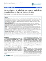
(iii) Examine a scree plot. This is a plot of the eigenvalues versus
the component number. The idea is to look for an “elbow”
which corresponds to the point after which the eigenvalues

decrease more slowly.
(iv) Consider whether the component has a sensible and useful
interpretation.
Winter Term 2013/14

15/24


Preliminaries
Methodology
Software
Applications

Choosing the number of components II
heptathlon_pca

2
1

Variances

3

4

●

●

●

●
●
●

6

7

0

●

1

2

3

4

5

Figure: Scree diagram for the principal components of the Olympic
heptathlon results.
Winter Term 2013/14

16/24

Preliminaries
Methodology
Software
Applications

Interpretation I
Correlations and covariances of variables and components
The covariance of variable i with component j is given by
Cov(xi , yj ) = ωj eji .
The correlation of variable i with component j is therefore
√
ωj eji
rxi ,yj =
,
si
where si is the standard deviation of variable i.
If the components are extracted from the correlation matrix,
then
√
rxi ,yj = ωj eji .
Winter Term 2013/14

17/24


Preliminaries
Methodology
Software
Applications

Interpretation II
Rescaling principal components
The coefficients ej an be rescaled so that coefficients for the
most important components are larger than those for less
important components.
These rescaled coefficients are calculated as
e∗j =

√

ωj ej ,

for which e∗j e∗j = ωj , rather than unity.
When the correlation matrix is analyzed, this rescaling leads
to coefficients that are the correlations between the
components and the original variables.
Winter Term 2013/14

18/24


Preliminaries
Methodology
Software
Applications

Rotation I
To enhance interpretation of the sample PCs, it is common in
PCA to rotate the matrix of loadings by optimizing a certain
“simplicity” criterion.

The method of rotation emerged in Factor Analysis and was
motivated both by solving the rotational indeterminacy
problem and by facilitating the factors’ interpretation.
Rotation can be performed either in an orthogonal or an
oblique (non-orthogonal) fashion.
Several analytic orthogonal and oblique rotation criteria exist
in the literature.
Winter Term 2013/14

19/24


Preliminaries
Methodology
Software
Applications

Rotation II

To aid interpretation, all rotation criteria are designed to make
the coefficients as simple as possible in some sense, with most
loadings made to have values either ‘close to zero’ or ‘far from
zero’, and with as few as possible of the coefficients taking
intermediate values.
After rotation, either one or both of the properties possessed
by PCA, that is, orthogonality of the loadings and
uncorrelatedness of the component scores, is lost.

Winter Term 2013/14

20/24


Preliminaries
Methodology
Software
Applications

PCA in the open-source software R

Function princomp() in the stats package:
Eigendecomposition of the covariance or correlation matrix.
Alternative: use directly the function eigen().

Function prcomp() in the stats package: SVD of the
(centered and possibly scaled) data matrix. Alternative: use
directly the function svd().

Winter Term 2013/14

21/24


Preliminaries
Methodology
Software
Applications

Air pollution in U.S. cities
High-dimensional data from the atmospheric science

Description of the data
For 41 cities in the United States the following seven variables
were recorded:
1

2
3

4
5
6
7

SO2 : Sulphur dioxide content of air in micrograms per cubic
meter
Temp: Average annual temperature in degrees Fahrenheit
Manuf : Number of manufacturing enterprises employing 20 or
more workers
Pop: Population size (1970 census) in thousands
Wind: Average annual wind speed in miles per hour
Precip: Average annual precipitation in inches
Days: Average number of days with precipitation per year

We shall examine how PCA can be used to explore various
aspects of the data.
Files: chap3usair.dat and pcausair.R
Winter Term 2013/14

22/24

Preliminaries
Methodology
Software
Applications

Air pollution in U.S. cities
High-dimensional data from the atmospheric science

Description of the data
Source: National Center for Environmental
Prediction/National Center for Atmospheric Research.
Winter monthly sea level pressures over the Northern
Hemisphere north of 20o N.
Gridded climate data with a 2.5o lat × 2.5o lon resolution
(p = 29 × 144 = 4176).
Period: December 1948 to February 2006. Winter season is
conventionally defined by December to February (n = 174).

Winter Term 2013/14

23/24


Preliminaries
Methodology
Software
Applications

Air pollution in U.S. cities
High-dimensional data from the atmospheric science

Spatial patterns
5

6

1

5

3

3

1

1

−1
1

1

−2

1

−3

−4

1

−1

−2

2

3
2

−1

−1

2
2

1

4

0

−2

2

3

−2 −3
1 −
1
5 4 2 1

1

−1

1
1

3

−1

2

−1

4

2 4
3
12

4

−1

1
0

1

−1
−2
−3

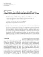
Figure: Spatial map representations of the two leading PCs for winter sea
level pressure data (left: North Atlantic Oscillation, right: North Pacific
Oscillation). The loadings have been multiplied by 100.

Winter Term 2013/14

24/24