An application of alternative risk measures to trading porfolios
Bạn đang xem bản rút gọn của tài liệu. Xem và tải ngay bản đầy đủ của tài liệu tại đây (441.35 KB, 37 trang )
Master Thesis: An Application of Alternative Risk Measures to Trading Portfolios
__________________________________________________________________________________________
-1-
An Application of Alternative Risk Measures to
Trading Portfolios
Master of Advanced Studies in Finance
ETH/Uni Zurich
30 January 2004
Abstract
This study covers the advantages of expected shortfall as an
alternative risk measure to value-at-risk and the results of implementing in
practice the tools of extreme value theory. EVT is applied to a varied sample
of trading portfolios across different sectors and sensitive to one and multiple
risk factors. A detailed analysis of the tail of the profit & loss empirical
distribution is performed with an emphasis on the estimates of value-at-risk
and expected shortfall. The concept of expected shortfall is also used as a
measure of sensitivity of the portfolio to risk factors, thus allowing to
determine the main drivers of risk.
Being involved with the market directly and on a daily basis, as well
as considering the recent events in the Russian market - more specifically, the
Yukos case, provided the opportunity to observe a real example when
historical VaR fails to be coherent.
Cornelia Glavan
Supervisor: Prof. Dr. Uwe Schmock Supervisor: Dr. Andreas Bitz
Institute for Financial and Head Market Risk Control
Actuarial Mathematics UBS Investment Bank
Vienna University of Technology Switzerland
Master Thesis: An Application of Alternative Risk Measures to Trading Portfolios
__________________________________________________________________________________________
-2-
Acknowledgements
A master thesis is often perceived as a result of an individual effort. This is hardly the case here, as the
following study is a result of a team work. The paper was written while doing an internship with the
Market Risk Control at UBS Investment Bank Zurich.
I am highly appreciative of the guidance and insights into the business from my supervisor Andreas Bitz
in particular, and the help from the whole Market Risk Control team in general. Sincere thanks to
Roberto Frassanito and Michael Rey for their most useful explanations and remarks.
I am very grateful to Prof. Uwe Schmock for all the help with the mathematical theory.
And last but not least, many thanks to all my friends and family for their help and support.
Master Thesis: An Application of Alternative Risk Measures to Trading Portfolios
__________________________________________________________________________________________
-3-
Contents
Abstract………………………………………………………………………………..1
Overview……………………………………………………………………………....4
1. Mathematical Theory…………………..…………………………………………..6
1.1 Expected Shortfall…………………..………………………………………….6
1.2 Generalized Pareto Distribution…….……………………………………..…...7
1.3 Method of Block Maxima……………………………………………………...9
1.4 Historical Approach ……...….…………………………………………….…10
2. Coherence and VaR…………………………………………………………....…11
2.1 Academic Example……………………………………………..…………….11
2.2 Practical Example: …...………………………………………………………11
2.3 Exploring the Tail………………………………………………………….…13
3. Equity Portfolios………………………………………………………………….15
3.1 One Risk Factor………………………………………………………………15
3.1.1 UBS stocks.……………………………………..………………….…15
3.1.2 Comparative analysis…………………………………….…………...17
3.2 Two Risk Factors…………………………………………………………….19
4. Currency and Fixed Income Portfolios: Multiple Risk Factors………………..…21
4.1 Currency portfolios……………………………………….….……………….21
4.2 Fixed Income Portfolios……………………………………………………...21
4.2.1 One Risk Factor: the Yield…………………………………………...22
4.2.2 Multiple Risk Factor..………………………………………………...23
5. Mixed Multiple Risk Factor Portfolio………..……………………………….….25
Conclusions: Why Expected Shortfall?…………………..…………….….…………29
References………………………..………………………….…………………….….30
Appendix B……………………………………………………………...………...…31
Appendix C…………………………………………………………….………….....32
Appendix D…………………………………………………………….………..…...34
Appendix E……………………………………………………………..………..…...36
Master Thesis: An Application of Alternative Risk Measures to Trading Portfolios
__________________________________________________________________________________________
-4-
Overview
Following Basel I rules, value-at-risk (VaR) has been established as one of the main risk
measures. Although widely used by financial institutions, the risk measure is heavily criticized in the
academic world for not being sub-additive, i.e. the risk of a portfolio as a whole can be larger then the
sum of the stand-alone risks of its components when measured by VaR. Consequently, VaR may fail to
justify diversification and does not take into account the severity of an incurred damage event. As a
response to these deficiencies, the notion of coherent risk measures was introduced. The most well
known coherent risk measure is expected shortfall (ES), which is the expected loss provided that the
loss exceeds VaR. A more detailed theoretical explanation is given in the first chapter, which comprises
the mathematical theory that is used in this paper. The current method at most financial institutions in
estimating VaR is based on a historical framework. In order to challenge this method, extreme value
theory (EVT) is used to estimate both value-at-risk and expected shortfall. The method of EVT focuses
on modelling the tail behaviour of a loss distribution using only extreme values rather than all the data.
This method, generalized Pareto distribution (GPD), has the theoretical background which allows fitting
the tail of the losses to a certain class of distributions.
The second chapter provides two examples demonstrating the advantages of expected shortfall
over VaR: the first is an artificial example, while the second is taken from practice and follows exactly
the framework currently used in estimating VaR at most financial institutions. The last example in this
chapter represents a practical case where extreme value theory can be used for financial data using a
different method, the one of block Maxima. This method is applied in order to give a better
understanding of event risk and is able to provide answers to questions like: "How rare is an event of
obtaining a return as low or lower than a certain loss?".
Further the paper contains the results of applying EVT to equity portfolios, currency portfolios
and fixed income portfolios. The third chapter discusses the results of applying EVT to equity portfolios
consisting of a single position: long stock and short stock. In these cases, we have only one risk factor -
the price log returns. To facilitate a better understanding of the behaviour of generalized Pareto
distribution when applied to equity portfolios, a representative collection of a wide range of stocks was
chosen: SMI and DAX, the well diversified European indices, Nasdaq - the much more volatile than its
European counter-parties American index. And the stocks of a highly liquid financial institution, and the
highly volatile stocks of ABB, Disetronic and Yukos, which have undergone a lot of distress in the time
period considered.
Next the analysis is done on positions of being long, short option on SMI. Two risk factors are
involved in these cases: the price log returns of the underlying and the absolute returns of the implied
volatility. EVT is applied in estimating the risk measure for the profit and loss function (P&L) when
risk factors are considered individually, as well as for the aggregated P&L. Given the multitude of risk
factors involved, historical P&L is preferred because it makes no assumptions about the correlation
between them.
The forth chapter discusses the results of estimating VaR and ES for some representative
portfolios from the currency and fixed income sectors.
In an attempt to cover a different gamut of currency portfolios, two low volatile cases
(JPY/USD and USD/EURO) and a highly volatile low liquidity case, characterized by an emerging
market currency USD/TRL, are considered. Generalized Pareto distribution is fitted to both the upper
and the lower tail of the distributions.
The chapter continues with a summary of the results of fitting the tail to GPD for fixed income
portfolio; two different bonds are considered. The main risk factors to which the P&L is mapped in the
first case is the spread to the Treasury curve, and the LIBOR curve and the spread in the second one.
The idea behind expected shortfall was used to measure the sensitivity of the aggregated P&L to the
moves of different risk factors.
Master Thesis: An Application of Alternative Risk Measures to Trading Portfolios
__________________________________________________________________________________________
-5-
The fifth chapter considers a hypothetical portfolio containing a variety of financial instruments
covering all the different businesses discussed in the paper. The historical approach is used to compute
the P&Ls mapped on different risk factors and expected shortfall is used as the main risk measure,
which allows us to make no assumptions about the correlation between risk factors and to make sure
that cases of incoherence are being avoided. The concept of expected shortfall is successfully used to
determine the main drivers of risk in the portfolio. This tool is employed to measure the sensitivity of
the overall portfolio to individual risk factors, thus allowing us to have a clear view of the risk and
potentially point to hedging strategies.
Master Thesis: An Application of Alternative Risk Measures to Trading Portfolios
__________________________________________________________________________________________
-6-
Chapter 1
Mathematical Theory
In this chapter the basic mathematical definitions necessary in understanding the paper are
given and also a detailed description of the methods used. One can skip this chapter now, provided that
while going through the paper you can then come back to check the notions used, given that links are
provided to find easier the parts of interest.
1.1 Expected Shortfall
Expected shortfall was proposed as an alternative risk measure to VaR, having the main
property of being coherent. In many articles different definitions for ES can be noticed, mainly coming
to the same one when we have the assumption that the distribution of the loss is continuous, differences
can appear when the distribution of the loss is no longer continuous. That is why it is important to have
strict definitions of expected shortfall and other risk measures. For those interested in exploring further
into this topic the article “On the Coherence of Expected Shortfall” by Carlo Acerbi and Dirk Tasche
provides all the necessary analytics and proofs used here, but not covered, which is beyond the purpose
of this paper.
Let X be a real-valued random variable (r.v.) on a fixed probability space. X is considered the
random profit of the portfolio, so we are mainly interested in losses, i.e. low values of X.
The exact mathematical definitions of some risk measures are given bellow:
α
- the confidence level (usually 0.95 or 0.99)
Definition 1
: Value-at-Risk: gives the maximum loss such that with a (1-
α
) probability we
exceed it.
}1][:inf{)(
α
α
−≥≤∈−= xXPRxXVaR
(1.1.1)
Observation: this is actually the lower (1-
α
)-quantile of X, taken with minus.
Definition 2
: Tail Conditional Loss: The expected loss provided that the loss exceeds VaR.
)(()( XVaRXXEXTCL
αα
−≤−=
) (1.1.2)
In some papers this is used as the definition for expected shortfall. But we need to be careful
about it, because this is the case when the distribution of the loss is continuous. The main property of
Expected shortfall is coherence, but using the definition as in the tail conditional loss (TCL) case, the
property of coherence is lost, as it is shown in the first example from the next chapter.
Before proceeding with the definition of expected shortfall, it is good to give the exact
characteristics of the property of coherence, especially that intuitively this property is expected to be
fulfilled by any function which gives us a number as a measure of risk. Before proceeding with the
concept of coherence we give the strict definition for a risk measure:
Definition 3
: Risk Measure
Let V be a set of real random variables on some probability space such that E[X
-
]
1
< ∞ for all
X∈V. Then a function ρ, which a gives a real number for any random variable in V is called a risk
measure. ρ: V → R
It is natural from a practical point of view to define coherence in the following way:
1
}0{
1
<
−
−=
X
XX
Master Thesis: An Application of Alternative Risk Measures to Trading Portfolios
__________________________________________________________________________________________
-7-
The property of Coherence: let ρ be a risk measure
(i) monotonous: X∈V , X ≤ 0, then
ρ
(X) ≥ 0
Given that a loss is certain to occur the risk function should exhibit this.
(ii) sub-additive: X, Y, X+Y∈V. then
ρ
(X+Y) ≤
ρ
(X) +
ρ
(Y)
The diversification effect: risk of a portfolio as a hole should be smaller then the sum of
the stand-alone risks of its components.
(iii) positively homogeneous: X∈V, h > 0, hX∈V then
ρ
(hX) = h
ρ
(X)
The risk is increasing proportionally with the magnitude of the portfolio, given the
weights of the assets stay the same.
(iv) translation invariant: X∈V, a – real number then
ρ
(X + a) = ρ(X) - a
If a certain gain (loss) is added to the portfolio, then its risk decreases (increases) with
the same amount as the gain (loss).
Definition 4
: Expected Shortfall:
)]))([)1)(((]1[(
1
1
)(
)}({
XVaRXPXVaRXEXES
xVaRX
ααα
α
α
α
−≤−−−
−
−=
−≤
(1.1.3)
As can be seen, by comparing ES with TCL, they are equal when the distribution of the loss is
continuous, so we may say that for continuous distributions TCL is coherent, problems arise when
dealing with cases in which P [X ≤ -VaR
α
(X)] ≠ 1-
α
.
Expected Shortfall is always coherent. An example showing us that VaR and TCL are not
coherent is provided in the second chapter. VaR on the other hand satisfies most of the properties of
being a coherent risk measure, except for the case of the sub-additive property. VaR is sub-additive for
example in the case when the distribution of X is elliptical, as it is the case of the normal and t-student
distributions
. For more details on the subject about the coherence of VaR for elliptical
distributions the reader is referred to [8].
1.2 Generalized Pareto Distribution
Extreme value theory goes back to the late 1920. But only recently it gained recognition as a
practical and useful tool in estimating tail risk. In the middle of the last century the econometricians
already discovered the non-normal behavior of financial markets, but this assumption is still widely
used in the financial industry, provided it is easy to implement. Using the EVT method we look only at
extreme losses and under the assumption that the losses occur independently we are also given the
theoretical background to use it. Here is discussed the generalized Pareto distribution used in estimating
the tail, this method is also referred to in many articles as peaks over threshold. A small theory is given
and also the Balkema and De Haan theorem on which the extreme value theory is constructed.
A threshold u is chosen, and then the losses, which lie beyond it are fitted to a GPD. The tools
of better choosing the threshold and the method to estimate the GPD used in this paper are discussed
further.
Let X
1
, X
2
, X
3
, …, X
n
be the losses. We make the assumption of them being independent and
identically distributed, and let F(x) = P (X
1
≤ x) be their distribution function.
Definition 5
: Let x
F
be the right end point of the distribution F
∞≤<∈= }1)(sup{ xFRxx
F
(1.2.1)
Master Thesis: An Application of Alternative Risk Measures to Trading Portfolios
__________________________________________________________________________________________
-8-
Definition 6: For any u < x
F
, we define the distribution function of the excesses over the
threshold u by
)(1
)()(
)()(
uF
xFuxF
uXxuXPxF
u
−
−+
=>≤−=
(1.2.2)
Comment: the choice of the threshold u being smaller then the right end point of the distribution
of the loss insures the fact that the probability of having a loss that exceeds it, is positive.
We can now discuss the maximum domain of attraction (MDA) conditions
MDA conditions
: Using all of the assumptions before, let
M
n
= max {X
1
, X
2
,…, X
n
}
Suppose that there exist the sequences of strictly positive numbers
Nnn
a
∈
)(
and a sequence of
real numbers
Nnn
b
∈
)(
such that the sequence of transformed maxima
n
n
nn
a
bM
)(
−
converges in
distribution.
)()( xHbxaFx
a
bM
P
n
nn
n
n
nn
ξ
→+=
≤
−
∞→
,for every continuity point x of H
ξ
,
(1.2.3)
where H
ξ
is a non-degenerate distribution function.
Comm ent: Reflecting on the MDA conditions the following question arises: “How does the
normalizing sequences
Nnn
a
∈
)(
and
Nnn
b
∈
)(
influence the limiting distribution H
ξ
,
?” The answer is that
the limit law is uniquely determined up to affine transformations. The proof is provided in the book
“Modelling Extremal Events for Insurance and Finance” by P. Embrechts, C. Klüppelberg and T.
Mikosch, theorem A1.5.
Now we are ready to write the fundamental theorem.
Theorem Balkema and De Haan
(1974)
Under the MDA conditions, the generalized Pareto distribution is the limiting distribution of
the excesses, as the threshold tends from below to the right-end point.
That is, there exists
β
(u) – positive function of u such that:
0)()(suplim
)(,
0
,
=−
−≤≤
→<
xGxF
uu
uxx
xuxu
F
FF
βξ
(1.2.4)
with G
ξ,β(u)
defined:
=−
≠+−
=
−
−
0,1
0,)
)(
1(1
)(
)(
1
)(,
ξ
ξ
β
ξ
β
ξ
βξ
u
x
u
e
u
x
xG
(1.2.5)
where: x ≥ 0 when ξ ≥ 0, and 0 ≤ x ≤ -
β
(u)/ ξ when ξ < 0.
We say that F belongs to the maximum domain of attraction of H
ξ
,
where H
ξ
is the generalized
extreme value distribution (GEVD):
=−
≠+−
=
−
−
0},exp{
0},)1(exp{
)(
1
ξ
ξξ
ξ
ξ
x
e
x
xH
(1.2.6)
where: 1+ξx > 0.
In fact this is the limiting distribution for transformed maxima from (1.2.3). The parameter ξ is
called the shape parameter, and it is an indicator of the fatness of the tail.
Master Thesis: An Application of Alternative Risk Measures to Trading Portfolios
__________________________________________________________________________________________
-9-
1.2.1 Properties of the tail of the distribution F:
If
ξ
>0, then we say that F belong to the MDA of the Fréchet distribution. Gnedenko showed
(1943) that the tail decays like a power function. In this class are heavy tail distributions like Pareto,
log-Gamma, Cauchy and t-student.
If
ξ
=0, then F is the MDA of the Gumbel distribution, this is the case of distributions where the
tail decays like the exponential function, examples: normal, exponential, and lognormal.
If
ξ
<0, this is the class of the Weibull distribution, in this case F has a support bounded above,
like the beta-distribution.
1.2.2 Tail fitting.
For x > u the upper tail distribution is the following:
)()())(1()( uXPuxFuXPxF
u
≤+−≤−=
(1.2.7)
from here, by taking F
n
(u) as the empirical probability of not exceeding the threshold (number of losses
smaller the u over the total number of losses) we can estimate the upper tail distribution:
)()())(1()(
,
uFxGuFxF
nn
+−=
βξ
(1.2.8)
It can be shown that F(x), for x > u can also be approximated with a GPD with the same shape
parameter
ξ
as for G
ξ
,
β
(u)
, the fitted GPD to the distribution of the excesses.
Method used to fit the tail:
We have a sample of iid (independent and identically distributed) losses x
1
, x
2
, x
3
, …, x
n
, then
we choose a threshold u and we look at extreme losses, those for which x
> u . Let’s assume there are k
losses bigger then u, and we write them as: x’
1
, x’
2
, …, x’
k
. Define y
i
= x’
i
– u, for every i from 1 to k.
Now we think of y
1
, y
2
,…, y
3
as being a sample from a GPD with parameters
ξ
,
β
which we want to
estimate.
We use the log-likelihood function in estimating the parameters. Under the assumption that
ξ
≠ 0, the log-likelihood function is:
∑
=
++−−=
k
i
i
y
kl
1
)]1ln()[
1
1()ln(),(
β
ξ
ξ
ββξ
and so in order to find
ξ
and
β
we maximize the log-likelihood function with the restrictions:
0>
ξ
and
0>
β
or
0<
ξ
and
ξβ
},...,max{
1 k
yy−>
.
Let
ξ
’ and
β
’ be the estimates obtained, then the estimate for the tail distribution
<−∈
>≥
−
+−=
−
0),,[
0,
,)
)(
1(1)(
1
ξ
ξ
β
ξ
β
ξ
ξ
whenuux
whenux
for
ux
n
k
xF
(1.2.8)
From here, since VaR
α
(α-the confidence interval) is the α-quantile, so VaR
α
=F
-1
(α). As to avoid any
confusions regarding VaR and Definition 1, here we say VaR is a quantile, because we estimate it from
the GPD, which is a continuous distribution. We say VaR
α
is the α-quantile and not (1-α)-quantile
because in this chapter we fit the tail distribution of losses, while in the first subchapter we considered
X - the profit. The obtained estimate for VaR
α
is:
n
k
provided
k
n
uaRV −≥−−+=
−
1,]1))1[((
α
ξ
β
α
ξ
α
(1.2.9)
And in the case of expected shortfall, since we look at the losses and the distribution is continuous:
)]()([)()]([)( XVaRXXVaRXEXVaRXVaRXXEXES
ααααα
>−+=>=
we obtain the estimate:
ξ
ββ
ξ
α
α
−
−
+
−
=
11
ˆ
ˆ
u
aRV
SE
, for the case
ξ
> 1 (1.2.10)
Master Thesis: An Application of Alternative Risk Measures to Trading Portfolios
__________________________________________________________________________________________
-10-
1.2.3 Mean Excess Function
As can been seen from the description above, we need to choose a threshold. What is the best
method in choosing it? On one hand the more points we have above the threshold, the more points we
have in estimating the tail, but on the other hand the theorem tells us the threshold should tend to the
right-end point.
In this case a good indicator in choosing the threshold is the mean excess plot. Suppose the
threshold excess X-u follows a GPD with parameters
ξ
and
β
, under necessary restrictions as in 1.2.5,
then
ξ
β
βξ
−
==>−
∫
1
)(][
,
xdGxuXuXE
(1.2.11)
For any u’>u we define the mean-excess plot as:
y
uuuu
uXuXEue
ξ
ξ
ξ
β
ξ
ξβ
−
+
−
=
−
−+
=>−=
11
)(
1
)'()(
]''[)'(
(1.2.12)
from the equality (1.2.7), it is seen that the mean-excess plot is a linear function of
y = u’-u. If we take the empirical mean-excess plot:
∑
=
−=
'
1
)(
'
)'(
1
)'(
u
n
i
i
u
n
ux
n
ue
, then, after plotting it for each u’, we choose u so that for
u’ > u it should look like a line. In most of the cases studied the conclusion was to choose u’ so that
95% of the sample points lie above u’.
1.3 Method of Block Maxima
In this paper a wide range of stocks are used and there will be cases in which the tail estimates
obtained seem to be sensible to some very extreme losses. And in this case a natural question arises: is
this loss an event risk? How rare is this loss and what is the probability of this happening again? EVT
can be successfully used to answer this question. And it even allows us to loosen the assumption of the
losses being independent. The general idea is to group the losses in blocks, like by month or quarter.
And then we fit the maximum losses from each block to the generalized extreme value distribution
(1.2.6). This is due to the Fisher-Tippett theorem (which tells us that if F (the distribution of losses)
belongs to the maximum domain of attraction then the block maxima follow a generalized extreme
value distribution.) The example when this method is used is provided in the second chapter, while here
we continue with a small description of the theory applied in it.
One of the important assumptions allowing for a fitting of block maxima
2
to a generalized
extreme value distribution (see 1.2.6) is the fact that the losses should be independent and identically
distributed. Further, the effects of relaxing the assumption of iid to consider just stationary processes
3
is
considered. With additional assumptions it can be shown that normalized block maxima indeed follow
a GEV distribution asymptotically.
We assume (X
n
) to be our stationary process, F the marginal distribution of X
i
, while (Y
n
) is the
associated iid process with the same marginal distribution F. The conditions necessary to be fulfilled by
(X
n
) such that the maxima of (X
n
) have exactly the same limiting behaviour as maxima of (Y
n
) are
as follows:
i) If the stationary series (X
n
) shows only weak long-range dependence, so that we can assume
that block maxima are independent.
ii) If it shows no inclination to form clusters of large values.
Then maxima of the two series have identical limiting behaviour.
2
in our cases monthly minimums will be considered as block maxima
3
a stationary process is one which is time invariant: for any h1 < h2 < … hn, and t > 0 we have that: (X
h1
, X
h2
, …,
X
hn
) = (in distribution)= (X
h1+t
, X
h2+t
, …, X
hn+t
)
Master Thesis: An Application of Alternative Risk Measures to Trading Portfolios
__________________________________________________________________________________________
-11-
Condition (i) is defendable for financial time series, while the anti-clustering condition is not.
Since the above theory is not applicable, a more detailed analysis of the issue of clustering is required.
For this purposes an extremal index of a stationary process is defined.
Definition 7
: Extremal index of a stationary process. (The intuition is that the maximum of n
observations from a stationary series with extremal index
θ
behaves like the maximum of n
θ
observations from the associated iid series.)
Let 0 ≤
θ
≤ 1 and suppose that for every τ > 0 there is a sequence of real numbers (u
n
(τ))
n>0
such
that:
ττ
→−
∞→n
n
uFn )))((1(
ϑτ
τ
−∞→
→≤ euMP
n
nn
)}({
Then we say that the stationary series (X
n
)
n>0
has the extremal index
θ
.
For more details, please see the paper by A. J. McNeil "Calculating Quantile Risk Measures for
Financial Return Series using Extreme Value Theory". The basic result used in the analysis follows:
Theorem 8
: Let (M
i
) the maximums if the stationary series (X
i
), and (L
i
) the maximums of (Y
i
)
(the associated iid series), and let
θ
>0 the extremal index of the stationary series, then:
)(}/){( xHxabLP
n
nnn
→≤−
∞→
for a non-degenerate H(x) if and only if
)(}/){( xHxabMP
n
nnn
θ
→≤−
∞→
with H
θ
(x) also non-degenerate.
This is the justification required to fit the GEVD to the block maxima of a stationary time
series, which shows the tendency of large values to form clusters.
We divide our series into k blocks with n observations in each block. Let (M
n
) be the
maxima of each block. Using the assumption that the maximas are independent, we fit them to
a generalized extreme value distribution. And using the maximum likelihood method we
estimate the parameters:
ξ, µ, σ of the GEV.
Where µ and σ are the location and scale parameters of
the extreme value distribution:
)()(
,,
σ
µ
ξσµξ
−
=
x
HxH
, where H
ξ
(x) is defined in 1.2.5
For more information about the maximum likelihood function used in estimating the parameters, the
reader is advised to see the book “Modelling Financial Time Series with S-PLUS” pag.130-143.
To avoid any confusions, we will use the following notations for the stationary series:
X-the loss, M-the maxima and F the marginal distribution. And for the associated iid series:
Y-the loss, L-the maxima and G the marginal distribution.
In the case when the sample is iid,
to estimate R
n,k
, the level we expect to exceed in one
block every k blocks, (the probability of having a return as low or lower then R
n,k
once in k
blocks is 1/k), we use that fact that R
n,k
is just the (1-1/k)-quantile of the distribution of block
maxima:
)(1}{1}{
1
.,,,, knknnknn
RHRLPRLP
k
σµξ
−=≤−=>=
The probability of obtaining a return as low or lower then
R
n,k
is 1-(1-1/k)
1/n
. Taking Y the
random variable representing the losses and G its marginal distribution:
n
knn
n
knknkn
k
RLPRGRYPRYP
/1
,
/1
,,,
)
1
1(1}{1)(1}{1}{ −−=≤−=−=≤−=>
Master Thesis: An Application of Alternative Risk Measures to Trading Portfolios
__________________________________________________________________________________________
-12-
However our losses are not iid, and in this case we use the extremal index and theorem 8 to
obtain an approximation of the probability of exceeding the return level
R
n,k
, where F is the marginal
distribution of our stationary series:
)(1)(1)(1)(1)(
,
)/(1
,
/1
,,, knn
n
knn
n
knknkn
RLPRMPRFRXPRXP ≤−=≤−=−=≤−=>
ϑ
)/(1
,
)/(1
)/11(1)(1
ϑϑ
n
knn
n
kRLP −−=≤−
An application of the above written theory is given in example 2.3.
1.4 Historical Approach
The historical simulation method consists of going back in time, such as over last 5 years and is
conceptually simple. We analyze the changes that have been seen in the risk factors over the specified
historical period. Then the portfolio under examination is then revalued, using the changes in the risk
factors, and so we construct the history of the hypothetical portfolio using current position. The
simulated P&L of the portfolio is obtained by taking daily simulated changes in the value of the
portfolio (the gain or loss of the portfolio, given that the positions stay unchanged and the next day the
market behaviors exactly as in the considered day).
The major advantages of the historical simulation is that the method is completely
nonparametric and does not depend on any assumptions about the distribution and correlations of the
risk factors. The method is robust and intuitive and, as such, forms the basis for the Basle 1993
proposals on market risks and is the most commonly used method in practice. But still the historical-
simulation method can be subject to some criticisms: only one path is used and the assumption is that
the past is a good estimate for what may happen in the immediate future.
The reader interested in detailed description of the method used in calculating the historical
simulated P&L is referred to book “Risk Management” by M. Grouphy, D. Galai and R. Mark, pag.206-
212
The empirical distribution of the loss is taken as the simulated historical P&L. In all the cases
considered, generalized Pareto distribution is fitted to the tail of the historical P&L and from it the
estimates for VaR and expected shortfall are drawn.
Historical VaR(α) is the (1-α)-quantile of the empirical distribution of the profit and loss. For
example when historical P&L is simulated over a time period of 5 years, then VaR(99%) is the 14
th
worse case. And historical ES(99%) is the average of the 14 losses bigger or equal to VaR(99%).
Master Thesis: An Application of Alternative Risk Measures to Trading Portfolios
__________________________________________________________________________________________
-13-
Chapter 2
Coherence and VaR
In order to demonstrate some of the affirmations mentioned in the previous chapter about
coherence, examples showing the advantages of expected shortfall over other risk measures are
provided below. This is also necessary as to better understand the intuition behind it.
2.1 An Academic Example
The following example entails two short positions in out-of-the-money binary options. The
specific details are shown in the table below. Each of our options has a 4% probability of a payout of -
100 CHF and a 96% probability of payout of zero, and the underlying variables of the two options are
independent of each other. If a VaR at the 95% confidence level is taken, than each of our positions has
a VaR of 0. However, if we combine the two positions, the probability of a zero payout falls to less than
95%, and so the VaR of the combined is positive (and, in this case, equal to 100 CHF)
4
. The VaR of the
combined position is therefore greater than the sum of the VaRs of the individual positions, so the VaR
is not sub-additive.
position Probability Payout VaR(95%)
5
TCL(95%)
6
ES(95%)
7
individual
0,04 -100
0,96 0
0
4
80
combined
0,0016 -200
0,0768 -100
0,9216 0
100
102
92
Table 2.1.1: Portfolios payoffs and their risk measures
VaR(X)+VaR(Y) < VaR(X+Y)
0
100
TCL(X)+TCL(Y) < TCL(X+Y)
8
102
ES(X)+ES(Y) > ES(X+Y)
160
92
Table 2.1.2
The table illustrates that neither VaR nor TCL are sub-additive, while ES is.
2.2 A Practical Example
The following real example is taken from emerging markets, although similar situations can be
encountered in developed markets as well. Given the recent events in the Russian markets, more
specifically - the Yukos affair, the following example was noticed.
4
a number for VaR of 100 means a loss of this magnitude.
5
Value-At-Risk at 99% confidence level
6
Tail Conditional Loss at 99% confidence level
7
Expected Shortfall at 99% confidence level
Master Thesis: An Application of Alternative Risk Measures to Trading Portfolios
__________________________________________________________________________________________
-14-
Let us consider the following two portfolios: the first one consists of 24 Yukos stocks, and the
other contains one stock of Sberbank. The method employed in calculating the P&L is the historical
approach and here we talk about historical VaR and historical ES. The time horizon considered is
February 7, 2003 to November 4, 2003. From February 7, 2003 forward the RTS – Russian Stock
Exchange Index - is calculated using the current methodology).
The graph bellow, plot 2.2.1 shows the scatter plot of the returns of Yukos's and Sberbank's
share prices. Looking closely to the plot, the returns from October 27, 2003 represents the VaR99 for
Sberbank returns and the worst case for Yukos returns (the graphical representation for it is the square),
while the one from October 30, 2003 is the VaR99 for the Yukos returns and the worst case for the
Sberbank returns (represented on the plot by a circle).
This is an unusual situation when the same date represents the date of the worst case for one
company and the VaR date for the other one, especially when considered that they are from different
industries: one is an oil giant and the second one is a commercial bank. But in this case we are dealing
with an amalgam of different factors. On October 27, 2003 the CEO of Yukos, Mikhail Khodorovsky
was arrested and on October 30, 2003 the Russian government has seized a controlling stake in Yukos.
These events, besides having a very strong negative impact on Yukos stock prices, sent strong
shock waves through the Russian stock market. This is a highly volatile and very poorly diversified
market. Out of the 59 companies listed on RTS (as from November 4, 2003) the largest six ones are all
fuel, metallurgy or energy companies, where Yukos has the biggest weight of about 21.69% as of
November 4, 2003
8
and the seventh company (according to market value) is Sberbank with a market
weight of 3.68%, all the other ones having a weight of less then 2%. In fact, the correlation coefficient
between Yukos and the RTS index over the same time horizon is 0.88, an extremely high one,
illustrating the weak diversification of the Russian market.
Sberbank Log Returns
-0,1
-0,05
0
0,05
0,1
-0,2 -0,1 0 0,1 0,2
Yukos Log Returns
Figure 2.2.1: scatter plot of Yukos and Sberbank log returns
8
The other five companies with the biggest weights are:
Surgutneftegas, fuel industry (13.69%)
LUKOIL, fuel industry (13.37%)
MMC “Norilsk Nickel”, metallurgy (9.11%)
Sibneft, fuel industry (8.17%)
United Energy System of Russia, electric energy (7.97%)