fluid mechanics and the theory of flight
Bạn đang xem bản rút gọn của tài liệu. Xem và tải ngay bản đầy đủ của tài liệu tại đây (7.52 MB, 225 trang )
R.S. Johnson
Fluid Mechanics and the Theory of Flight
Download free eBooks at bookboon.com
2
Fluid Mechanics and the Theory of Flight
© 2012 R.S. Johnson & Ventus Publishing ApS
ISBN 978-87-7681-975-0
Download free eBooks at bookboon.com
3
Fluid Mechanics and the Theory of Flight
Contents
Contents
Preface
7
1
Introduction and Basics
8
1.1
he continuum hypothesis
9
1.2
Streamlines and particle paths
10
1.3
he material (or convective) derivative
14
1.4
he equation of mass conservation
18
1.5
Pressure and hydrostatic equilibrium
23
1.6
Euler’s equation of motion (1755)
25
Exercises 1
29
2
Equations: Properties and Solutions
38
2.1
he vorticity vector and irrotational low
38
2.2
Helmholtz’s equation (the ‘vorticity’ equation)
42
2.3
Bernoulli’s equation (or theorem)
44
2.4
he pressure equation
48
2.5
Vorticity and circulation
52
2.6
he stream function
56
2.7
Kinetic energy and a uniqueness theorem
59
Exercises 2
61
e Graduate Programme
for Engineers and Geoscientists
I joined MITAS because
I wanted real responsibili
Maersk.com/Mitas
Real work
International
Internationa
al opportunities
work
ree wo
or placements
Month 16
I was a construction
supervisor in
the North Sea
advising and
helping
foremen
he
ssolve problems
Download free eBooks at bookboon.com
4
Click on the ad to read more
Fluid Mechanics and the Theory of Flight
Contents
3
Viscous Fluids
67
3.1
he Navier-Stokes equation
67
3.2
Simple exact solutions
68
3.3
he Reynolds number
75
3.4
he (2D) boundary-layer equations
77
3.5
he lat-plate boundary layer
81
Exercises 3
84
4
Two dimensional, incompressible, irrotational low
88
4.1
Laplace’s equation
88
4.2
he complex potential
90
4.3
Simple (steady) two-dimensional lows
91
4.4
he method of images
109
4.5
he circle theorem (Milne-homson, 1940)
113
4.6
Uniform low past a circle
116
4.7
Uniform low past a spinning circle (circular cylinder)
119
4.8
Forces on objects (Blasius’ theorem, 1910)
121
4.9
Conformal transformations
128
4.10
he transformation of lows
131
Exercises 4
134
www.job.oticon.dk
Download free eBooks at bookboon.com
5
Click on the ad to read more
Fluid Mechanics and the Theory of Flight
Contents
5
Aerofoil heory
140
5.1
Transformation of circles
141
5.2
he lat-plate aerofoil
148
5.3
he lat-plate aerofoil with circulation
153
5.4
he general Joukowski aerofoil in a low
159
Exercises 5
163
Appendixes
165
Appendix 1: Biographical Notes
165
Appendix 2: Check-list of basic equations
184
Appendix 3: Derivation of Euler’s equation (which describes an inviscid luid)
186
Appendix 4: Kelvin’s circulation theorem (1869)
189
Appendix 5: Some Joukowski aerofoils
190
Appendix 6: Lit on a lat-plate aerofoil
191
Appendix 7: MAPLE program for plotting Joukowski aerofoils
193
Answers
194
Index
209
Download free eBooks at bookboon.com
6
Click on the ad to read more
Fluid Mechanics and the Theory of Flight
Preface
Preface
his text is based on lecture courses given by the author, over about 40 years, at Newcastle University, to inal-year applied
mathematics students. It has been written to provide a typical course that introduces the majority of the relevant ideas,
concepts and techniques, rather than a wide-ranging and more general text. hus the topics, with their detailed discussion
linked to the many carefully worked examples, do not cover as broad a spectrum as might be found in other, more wideranging texts on luid mechanics; this is a quite deliberate choice here. hus the development follows that of a conventional
introductory module on luids, comprising a basic introduction to the main ideas of luid mechanics, culminating in a
presentation of complex-variable techniques and classical aerofoil theory. (here are many routes that could be followed,
based on a general introduction to the fundamentals of the theory of luid mechanics. For example, the course could then
specialise in viscous low, or turbulence, or hydrodynamic stability, or gas dynamics and supersonic low, or water waves, to
mention just a few; we opt for the use of the complex potential to model lows, with special application to simple aerofoil
theory.) he material, and its style of presentation, have been selected ater many years of development and experience,
resulting in something that works well in the lecture theatre. hus, for example, some of the more technical aspects are
set aside (but usually discussed in an Appendix).
It is assumed that the readers are familiar with the vector calculus, methods for solving ordinary and partial diferential
equations, and complex-variable theory. Nevertheless, with this general background, the material should be accessible to
mathematicians, physicists and engineers. he numerous worked examples are to be used in conjunction with the large
number of set exercises – there are over 100 – for which the answers are provided. In addition, there are some appendices
that contain further relevant material, together with some detailed derivations; a list of brief biographies of the various
contributors to the ideas presented here is also provided.
Where appropriate, suitable igures and diagrams have been included, in order to aid the understanding – and to see the
relevance – of much of the material. However, the interested reader is advised to make use of the web, for example, to
ind pictures and movies of the various phenomena that we mention.
Download free eBooks at bookboon.com
7
Fluid Mechanics and the Theory of Flight
Introduction and Basics
1 Introduction and Basics
We start with a working deinition: a luid is a material that cannot, in general, withstand any force without change of
shape. (An exception is the special problem of a uniform – inward – pressure acting on a liquid, which is a luid that
cannot be compressed, so there is no change of volume.) his property of a luid should be compared with what happens
to a solid: this can withstand a force, without any appreciable change of shape or volume – until it fractures!
We take this fundamental and deining property as the starting point for a simple classiication of materials, and luids
in particular:
materials
solids
?
fluids
low density gases
liquids
(incompressible)
viscous
(real)
inviscid
(m odel/
ideal)
ga ses
(compressible)
viscous
(real)
inviscid
(model/
ideal)
(Some materials sit somewhere between solids and luids; these are usually called thixotropic materials – non-drip paints
are an example.)
We are interested in luids, of which there are two main types exempliied by: air – a gas – which is easily compressed
(until it liqueies), whereas water – a liquid – is virtually incompressible. (he density of water increases by about 0 ⋅ 5%
under a pressure of 100 atmospheres.)
All conventional luids are viscous; simply observe the various phenomena associated with the stirred motion of a drink
in a cup; e.g. ater stirring, the motion eventually comes to a halt; also, during the motion, the particles of luid directly
in contact with the inner surface of the cup are stationary.
In this study, we will eventually work, mainly, with a model luid that is incompressible. his applies even to air – relevant
to the theory of light – provided that the speeds are less than about 300mph (which is certainly the situation at take of
and landing). he rôle of viscosity is important in aerofoil theory, and will therefore be discussed carefully, but it turns
out that the details of viscous low are not signiicant for light.
Download free eBooks at bookboon.com
8
Fluid Mechanics and the Theory of Flight
Introduction and Basics
1.1 The continuum hypothesis
he irst task is to introduce a suitable, general description of a luid, and then to develop an appropriate (mathematical)
representation of it. his involves regarding the body of luid on the large (macroscopic) scale i.e. consistent with the
familiar observation that luid – air or water, for example – appears to ill completely the region of space that it occupies:
we ignore the existence of molecules and the ‘gaps’ between them (which would constitute a microscopic or molecular
model). his crucial idealisation, which regards the luid as continuously distributed throughout a region of space, is called
the continuum hypothesis.
Now, at every point (particle), we may deine a set of functions that describe the properties of the luid at that point:
u(x, t ) – the velocity vector (a vector ield)
p (x, t ) – the pressure (a scalar ield)
ρ (x, t )
– the density (ditto),
x = ( x, y, z ) is the position vector (expressed in rectangular Cartesian coordinates, but other coordinate systems
may sometimes be required). Here, t is time and we usually write u = (u , v, w) , although there may be situations where
the components are more conveniently written as xi and ui ( i = 1, 2,3 ). Note that both p and ρ are deined at a
where
point, with no preferred orientation: they are isotropic. Also, we have not included temperature, the variations of which
may be important for a gas (requiring a consideration of thermodynamics and the introduction of thermal energy). We
will mention temperature only as a consequence of other properties e.g. pressure and density implies a certain temperature,
via some equation of state. We assume, for our discussion here, that all the motion occurs at ixed temperature throughout
the luid, or that heat transfer between regions of diferent temperature can be ignored (e.g. it occurs on timescales far
longer than those associated with the low under consideration).
In our initial considerations, we shall allow the density to vary, but we will soon revert to the appropriate choice for our
incompressible (model) luid:
ρ = constant . Further, the three functions introduced above are certainly to be continuous
in both x and t for any reasonable representation of a physically realistic low.
Note: his description, which deines the properties of the luid at any point, at any time – the most common one in
use – is called the Eulerian description. he alternative is to follow a particular point (particle) as it moves in the luid,
and then determine how the properties change on this particle; this is the Lagrangian description. We shall write more
of these alternatives later.
Download free eBooks at bookboon.com
9
Fluid Mechanics and the Theory of Flight
Introduction and Basics
We are now in a position to introduce two diferent ways of describing the general nature of the motion in a given velocity
ield which represents a luid low.
1.2 Streamlines and particle paths
We assume that we are given the velocity ield
u(x, t ) (and how any particular motion is generated or maintained is, for
the moment, altogether irrelevant); the existence of a motion is the sole basis for the following descriptions.
1.2.1 A streamline is an imaginary line in the luid which everywhere has the velocity vector as its tangent, at any instant
in time.
Let such a curve be parameterised by s, and write the curve as
x = X( s, t ) ; we give a reminder of the underlying idea
that we now use.
u
u
∆X
X( s + ∆s, t )
= X( s, t ) + ∆X
X(s,t)
O
dX
X( s + ∆s, t ) − X( s, t ) ∆X
, so that, in the limit ∆s → 0 , the derivative
is the tangent to the curve
=
ds
∆s
∆s
x = X( s, t ) – a familiar result. hus our deinition of a streamline can be expressed as
We form
dX
dX
dX
∝ u or
= ku or
= u( X, t ) ,
ds
ds
ds
when we redeine s. In Cartesian components, this is the set of three coupled, ordinary diferential equations
dx
dy
dz
= u,
= v,
= w (all at ixed t)
ds
ds
ds
or, more conveniently, a pair of equations e.g.
dy v d z w
= ,
= .
dx u dx u
Download free eBooks at bookboon.com
10
Fluid Mechanics and the Theory of Flight
Introduction and Basics
his set is oten expressed in the symmetric form
dx dy dz
=
= .
u
v
w
Note that, in 2-space (x, y), we simply have
dy v
=
dx u
(because there is no variation, and no low, in the z-direction).
Example 1
Streamlines. Find the streamlines for the low
u ≡ (α xt ,−α y,0) , where α > 0 is a constant, and that family
at the instant t = 1 .
igure).
We have (in 2D)
hus
dy v
αy
y
= =−
= − (at ixed t; x ≠ 0, t ≠ 0 ), and so
dx u
xt
α xt
dy
dx
t∫
= −∫
i.e. t ln y = − ln x + constant .
y
x
y t x = C (an arbitrary constant), and then at t = 1 we have simply xy = C (a family of rectangular hyperbolae;
see igure).
Comment: Streamlines cannot cross except, possibly, where u = 0 (deining a stagnation point, where the low is stationary
or stagnant) because, at such points, the direction of the zero vector is not unique.
1.2.2 A particle path is the path,
x = X(t ) , followed by a point (particle) as it moves in the luid according to the given
velocity vector i.e.
dX
=u;
dt
Download free eBooks at bookboon.com
11
Fluid Mechanics and the Theory of Flight
this is pure kinematics, determining
Introduction and Basics
X(t ) given u( X, t ) . In component form, we have
dx
dy
dz
=u,
=v,
= w,
dt
dt
dt
and here t is a variable (involved in the integration process).
Example 2
Particle paths. Find the particle paths for the low
u ≡ (α xt ,−α y,0) , and that path which passes through
(1,2) at .
Here we have
dx
dy
dz
= α xt ,
= −α y (and
= 0 ⇒ z = constant , so 2D); thus
dt
dt
dt
dx
dy
2
∫ x = α ∫ t dt; ∫ y = −α ∫ dt i.e. ln x = 12 α t + const.; ln y = −α t + const.
1
which gives
(
1
x(t ) = e 2
αt 2
x = Ae 2
αt 2
; y = Be−α t and data at t = 0 requires A = 1, B = 2 . he path is therefore
)
, 2e −α t , const. , when expressed in 3D.
Join the Vestas
Graduate Programme
Experience the Forces of Wind
and kick-start your career
As one of the world leaders in wind power solutions with wind turbine installations in over 65
countries and more than 20,000 employees
globally, Vestas looks to accelerate innovation
through the development of our employees’ skills
and talents. Our goal is to reduce CO2 emissions
dramatically and ensure a sustainable world for
future generations.
Read more about the Vestas Graduate
Programme on vestas.com/jobs.
Application period will open March 1 2012.
Download free eBooks at bookboon.com
12
Click on the ad to read more
Fluid Mechanics and the Theory of Flight
Introduction and Basics
Note: A steady low is one for which the velocity ield is independent of time, and then the families of streamlines (SLs)
and particle paths (PPs) necessarily coincide (because
dX
dX
= u( X) and
= u( X) each deine the same set of curves).
ds
dt
Example 3
Steady low. All the particles (points) in a luid move according to
x ≡ ( aet , be2 t , ce −3t )
(written in rect.
Cart. coords.). Show that this low ield is steady, and then that the families of SLs and PPs coincide.
dx
(
−3t
)
= ae , 2be , −3ce
he PPs are given, and so u =
; but these PPs can be expressed as x(t ) = ( x(t ), y (t ), z (t )) ,
dt
t
where x(t ) = ae , etc., and so eliminating a, b, c we obtain the velocity ield u = ( x, 2 y, −3 z ) for all particles (points)
t
2t
in the low. his velocity ield is steady.
dx dy
dz
and so for example – other choices are possible –
=
=
x 2 y −3 z
a2
y, y 3 z 2 = b3e6t c 2e−6t = b3c 2 ,
x 2 = Ay, y 3 z 2 = B ; but the PPs give x 2 = a 2e 2t =
b
Now the SLs are
which is consistent with the representation of the SLs: the two families coincide.
Example 4
nt
SLs and PPs II. he velocity components of a low (in 2D) are ( xye , y ) ( ≡ u ) , where t is time and n is a
constant. Find the streamlines for this low and the particle path which passes through (1,1) at t = 0. For what
value of n will the two families of curves coincide ?
dx
dy
= u = xye nt ,
= v = y , and so we must solve the second equation irst:
dt
dt
ln y = t + const. i.e. y = Aet = et to satisfy the initial condition. hen
We have, for the PPs,
dx
= xe(1+ n)t :
dt
∫
1 (1+ n)t
e(1+ n)t − 1
dx
(1+ n )t
+ const. =
;
∫ x = ∫ e dt so ln x = 1 + n e
1+ n
e(1+ n)t − 1
thus x = exp
.
1 + n
Download free eBooks at bookboon.com
13
dy
= dt so
y ∫
Fluid Mechanics and the Theory of Flight
For the SLs:
∫
Introduction and Basics
dy v
y
1
( x ≠ 0, y ≠ 0 ), and so
= =
=
dx u xyent xent
dx
= ent ∫ dy (at ixed t) i.e. ln x = yent + const. or x = C exp ye nt .
x
( )
he two families coincide for steady low i.e. n = 0 .
Comment: In the laboratory, it is sometimes convenient to observe streak lines; these are all the paths through a given
point, over an interval of time.
1.3 The material (or convective) derivative
Let us consider some (scalar) property of the luid, labelled f ; in our representation of a luid, this will be the pressure,
or the density or a velocity component. his will, in general, vary in position and time:
f = f (x, t ) .
∂f
, but a more important aspect of f is how it varies in time when it is associated with a point
∂t
df
dX
(particle) that is moving in the luid. So we require
with
= u ; then we have
dt
dt
We might be interested in
d
dX
∂f
∂
{ f ( X(t ), t )} = + ⋅∇ f = + u ⋅∇ f
dt
∂t dt
∂t
,
and this operator on f is called the material (or convective) derivative (because it gives the rate of change of a material
point – a point or particle of the material, as it moves, or is ‘convected’, in the luid); it is usually written as
D ∂
≡ + u ⋅∇ .
Dt ∂t
Download free eBooks at bookboon.com
14
Fluid Mechanics and the Theory of Flight
Introduction and Basics
Warning:
Do not think to write u ⋅∇ as ∇ ⋅u ! Remember that ∇ is a diferential operator and so, in the former, it
operates on whatever follows the ∇ , and this is not u – it is some function e.g. f.
Note: If we apply this operator to the velocity vector – which we might expect is the appropriate representation of the
acceleration of a luid particle – then we obtain
D u ∂u
=
+ (u ⋅∇)u ,
Dt ∂t
which is inherently nonlinear. hat this is indeed the acceleration follows directly: we have
and so the acceleration is
d2X
dt 2
=
dX
= u for a particle path,
dt
d
Du
∂u dX
+
⋅∇u =
u( X(t ), t ) =
,
dt
Dt
∂t dt
relating the Lagrangian and Eulerian expressions.
In Paris or Online
International programs taught by professors and professionals from all over the world
BBA in Global Business
MBA in International Management / International Marketing
DBA in International Business / International Management
MA in International Education
MA in Cross-Cultural Communication
MA in Foreign Languages
Innovative – Practical – Flexible – Affordable
Visit: www.HorizonsUniversity.org
Write:
Call: 01.42.77.20.66
www.HorizonsUniversity.org
Download free eBooks at bookboon.com
15
Click on the ad to read more
Fluid Mechanics and the Theory of Flight
Introduction and Basics
Example 5
Acceleration. Find the acceleration vector for a particle (point) which moves according to
two dimensions, where α > 0
We have
u ≡ (αx ,−αy ) , in
is a constant.
u = α x, v = −α y (& w = 0) , so
D ∂
∂
∂
≡ + α x − α y ; thus
Dt ∂t
∂x
∂y
∂
∂
∂
∂
Du ∂u
=
+ α x − α y u = α x − α y (α x, −α y ) = α 2 x, α 2 y
∂y
∂y
Dt ∂t ∂x
∂x
(
)
.
he notion of acceleration can be explored further:
Example 6
Velocity & Acceleration. A particle starts (t = 0) at the point (a, b, c), and moves according to
x = ( x, y, z ) = a(1 + t )2 , b (1 + t ) , c (1 + t ) . Find the velocity and acceleration vectors directly;
(
)
determine the velocity ield in terms of x, y, z and t (by eliminating a, b and c), and hence show that the
acceleration is recovered from
We have
Du Dt .
dx
b
c
,
= 2a (1 + t ), −
−
=u;
dt
(1 + t ) 2 (1 + t ) 2
correspondingly,
the acceleration is
2b
2c
2
a
,
,
=
.
dt 2
(1 + t )3 (1 + t )3
d 2x
y
z
2x
,−
,−
for this velocity ield i.e. for every point satisfying the given family of PPs;
1+ t 1+ t 1+ t
But we may write u =
this low ield is therefore unsteady.
Download free eBooks at bookboon.com
16
Fluid Mechanics and the Theory of Flight
Now
Introduction and Basics
Du ∂
2x ∂
y ∂
z ∂
= +
−
−
u
Dt ∂t 1 + t ∂x 1 + t ∂y 1 + t ∂z
y
y
z
z
2x
4x
2b
2c
a
= −
+
+
+
=
,
,
2
,
,
(1 + t ) 2 (1 + t ) 2 (1 + t ) 2 (1 + t ) 2 (1 + t ) 2 (1 + t ) 2
(1 + t )3 (1 + t )3
exactly as before.
Download free eBooks at bookboon.com
17
Fluid Mechanics and the Theory of Flight
Introduction and Basics
1.4 The equation of mass conservation
A fundamental equation (not usually expressed explicitly in elementary particle mechanics) is a statement of mass
conservation. We can readily see the need for such an equation: the luid is, in general, in motion and can produce a
mixing of regions of diferent densities. Yet the total amount (mass) of material is presumably conserved; this total can
change only if matter (material) is created or destroyed – and this will arise only if we allow e.g. the conversion of mass
into energy! We now derive the equation which ensures that mass is indeed conserved.
Consider an imaginary (inite) volume V, bounded by a surface S, which is completely occupied by luid; we shall take V
(and S) to be stationary in our chosen frame of reference (so that luid will cross S into and out of V). his igure shows
the coniguration schematically:
where n is the outward unit normal on S, and
ρ (x, t )
and
u(x, t ) are given at every point in V and on S. he total
mass of all the luid in V, at any instant in time, is then
∫ ρ (x, t ) dv ,
V
where
∫ (.) dv denotes the triple integral in x over V. he rate of change of this mass is therefore
V
d
∂ρ
ρ (x, t ) dv = ∫
dv
∫
dt
∂t
V
V
because V is ixed in space. [See the property: ‘diferentiation under the integral sign’, discussed in Exercise 10.]
Download free eBooks at bookboon.com
18
Fluid Mechanics and the Theory of Flight
Introduction and Basics
Further, the net rate at which mass lows out of V across S is described in this igure:
length is
l = u ⋅n
per unit time
∆S
u
and so the volume of luid (out) per unit time is approximately l × ∆S = u ⋅ n∆S , producing a total mass low rate
(out), over all S, in the form
∫ ρu ⋅ n ds ,
S
where
∫ (.) ds represents the double integral over S. We now impose the condition that the only mechanism that produces
S
a change of mass in V is by virtue of material crossing S (into or out of V), thereby excluding the possibility of matter
(mass) being created or destroyed at any points in V or on S; thus we require
∂ρ
∫ ∂t dv = − ∫ ρu ⋅ n ds .
V
S
he choice of sign here is to accommodate the obvious convention that
∂ρ
> 0 requires material to enter V across S.
∂t
We now invoke the Divergence (Gauss’) heorem for the surface integral (where S bounds V), to produce
∂ρ
∫ ∂t + ∇ ⋅ ( ρu) dv = 0 .
V
However, this result must hold for all Vs (and corresponding Ss), irrespective of shape or size, which implies that the
limits of the integral (denoted by V) are arbitrary. But
∂ρ
+ ∇ ⋅ ( ρ u) is assumed continuous, and so the requirement
∂t
that the integral of this expression always be zero [see the fundamental idea discussed in Exercise 11] gives
∂ρ
+ ∇ ⋅ ( ρ u) = 0
∂t
Download free eBooks at bookboon.com
19
Fluid Mechanics and the Theory of Flight
Introduction and Basics
which is usually expressed [see the identities in Exercise 7] as
Dρ
+ ρ∇ ⋅ u = 0 ,
Dt
the equation of mass conservation for a general luid. Immediately we see that, if
ρ = constant (> 0) , then we obtain
∇ ⋅u = 0
which is a statement that volume is conserved. Note that the equation of mass conservation requires both ρ and u to be
diferentiable.
In rectangular Cartesian coordinates, ∇ ⋅ u = 0 becomes
with
u = (u , v, w) , this reads
∂u ∂v ∂w
+ +
= 0 ; in cylindrical polar coordinates (r , θ , z ) ,
∂x ∂y ∂z
1 ∂ (ru ) 1 ∂v ∂w
+
+
= 0.
r ∂r
r ∂θ ∂z
A check list of all the relevant equations, written in both rectangular Cartesian coordinates and cylindrical coordinates,
is given in Appendix 2.
Note: he general deinition of an incompressible luid is that ρ = constant on each luid particle (allowing diferent
constants on diferent particles), so that Dρ = 0 , leaving the same result as above: ∇ ⋅ u = 0 . Our usual choice, appropriate
Dt
for a conventional incompressible luid, is a special solution of this system: ρ = constant everywhere. he equation
∇ ⋅ u = 0 simply states that volume is conserved (which we could have derived directly, if we wished to limit our
discussion to incompressible luids).
Comment: We observe that, in the case where
∂ρ
+ ∇ ⋅ ( ρ u) is not continuous, the integral representing mass
∂t
conservation recovers a jump condition deining the relation between low properties on either side of the discontinuity.
In the context of a gas, this describes conditions across a shock wave in supersonic low.
Example 7
Incompressible low. A low is described by the velocity ield
the constants
α , β ,γ
We have directly that ∇ ⋅ u = u x
thus
α + β +γ = 0
u ≡ (αx, βy, γz ) ; what relation must exist between
for this to represent an incompressible low ?
+ v y + wz = α + β + γ (where subscripts have been used to denote partial derivatives);
is the condition for this velocity ield to represent an incompressible low.
Download free eBooks at bookboon.com
20
Fluid Mechanics and the Theory of Flight
Introduction and Basics
A more interesting example, leading to an important, simple result used in elementary calculations for low along a pipe,
is the following:
Example 8
Pipe low. An incompressible low, which is axisymmetric and non-swirling, moves along a circular pipe of
varying cross-section (radius R(z)). Find the relation between speed along the pipe and its cross-sectional area.
For incompressible low in cylindrical coordinates, we have
1∂
1 ∂v ∂w
(ru ) +
+
= 0 ; then for axisymmetry ( ∂ ∂θ ≡ 0 ) and no swirl ( v ≡ 0 ), this reduces to
r ∂r
r ∂θ ∂z
1∂
∂w
(ru ) +
= 0 (and note that either condition removes this term, but the irst also ensures that no functions
∂z
r ∂r
depend on θ). We write this equation as ( ru ) r + ( rw) z = 0
and then integrate across the pipe:
R( z )
[ ru ]0
R( z )
+
∫
(rw) z dr = 0 .
0
We now invoke the ‘diferentiation under the integral sign’ ( Exercise 10) to express this as
R( z )
0
[ ru ]
but ru = 0 on r = 0 , so this becomes
d
+
dz
R( z )
∫
0
rw dr − Rw r = R R′ = 0
R (u − wR′) r = R +
Download free eBooks at bookboon.com
21
d
dz
R( z )
∫
0
rw dr = 0 .
Fluid Mechanics and the Theory of Flight
Introduction and Basics
here are two cases of interest: irst, for a viscous luid, both u and w are zero at the inner surface of the pipe (because
there can be no low through the pipe, nor along the pipe), and so the evaluation on
r = R ( z ) gives zero. On the other
hand, we might suppose that the luid can be modelled as inviscid (zero viscosity – no friction), in which case the luid
is allowed to low along the inside surface of the pipe (but, as before, not through it). In this case, we must have that
the velocity vector is parallel to the pipe wall i.e.
d
hus
dz
R( z )
∫
0
rw dr = 0 and so
(u w) r = R = R′( z ) , and again the evaluation on r = R ( z ) is zero.
R( z )
∫
rw dr = constant , the required result.
0
In the special case (e.g. a model) in which the velocity proile across the pipe is essentially independent of the radius (r),
the integral produces the rule: speed×area = constant. his type of low is usually referred to as uniform across a section,
as depicted for a real low which is nearly uniform across a section in the igure.
Are you remarkable?
Win one of the six full
tuition scholarships for
International MBA or
MSc in Management
Download free eBooks at bookboon.com
22
register
now
rode
www.Nyen
ge.com
n
le
MasterChal
Fluid Mechanics and the Theory of Flight
Introduction and Basics
1.5 Pressure and hydrostatic equilibrium
We now introduce the initial ideas that will, eventually, lead to an equation of motion – the corresponding Newton’s
Second Law – for a luid. he irst stage is to discuss the forces that act on a luid; there are three (although we shall put
one of these aside, for the moment):
• force due to pressure (force/area), exerted by the luid particles nearby
• internal friction (viscous forces) due to motion of other particles nearby
• external force (body force) that acts more-or-less equally on all luid particles e.g. gravity.
he irst two in this list are internal, local forces; in this discussion, we shall ignore any friction (and, in any event, there
will be no motion, so friction cannot play any rôle). he pressure,
p (x, t ) , is deined at every point in the luid, and is
independent of orientation (the luid is said to be isotropic). Under the action of pressure and a body force – gravity,
perhaps – the luid is in equilibrium; we now construct the equation that describes this scenario.
As before, let us consider an imaginary volume V, surface S, with outward normal n and totally occupied by luid. Let
the body force acting on the luid be
F (x, t ) per unit mass; the pressure (due to the surrounding luid) acts on S.
pn∆S
S
v
V
ρ F∆V
he total body force acting on all the luid in V is thus
∫ ρ Fdv ;
V
correspondingly, the total pressure force acting on S is
− ∫ pnds .
S
here are no other forces acting, and there is no motion, so the resultant force on the luid must be zero (the luid is in
equilibrium under the action of these forces) i.e.
∫ ρ Fdv − ∫ pnds = 0 .
V
S
Download free eBooks at bookboon.com
23
Fluid Mechanics and the Theory of Flight
Introduction and Basics
(Note that the force, as expressed by the let-hand side, is force on.)
Again, we use the Divergence (Gauss’) heorem, to give (for the second term)
∫ pnds = ∫ ∇pdv (see Exercise 8),
S
and so we obtain
V
∫ ( ρ F − ∇p ) d v = 0 .
V
For this to be valid for all possible choices of V (and associated S), and for a continuous integrand, we require
ρ F − ∇p = 0 or ∇p = ρ F ;
this is the equation of hydrostatic equilibrium (because water is a special case!).
Note that the density here, ρ, is not necessarily a constant: we have made no assumptions about ρ or the nature of the
luid under discussion.
Example 9
Hydrostatic equilibrium. Given that the body force is due to (constant) gravity, so that
that the pressure
F ≡ (0,0,− g ) , and
p = p0 on z = 0 , ind p (z ) for an incompressible luid (i.e. ρ = constant) in hydrostatic
equilibrium.
∂p ∂p ∂p
∂p
∂p
∇p = ρ F i.e. , , = ρ (0, 0, − g ) , and so
= 0,
= 0 , which gives
∂x
∂y
∂x ∂y ∂z
p = p ( z ) . hen p′( z ) = − ρ g , and so p = p0 − ρ gz .
he governing equation is
Comment: On the basis of the previous example, if z = 0 is the surface of the ocean, then the pressure increases linearly
with depth. On the other hand, if z = 0 is the bottom of the atmosphere, then the pressure decreases linearly with height
(but this is not a good model for the atmosphere – compressibility is important, with
p = p ( ρ ) ).
In this model, also note that the rate of increase/decrease is very diferent for water/air, because of the very diferent
densities; for example, the pressure drops to about half an atmosphere at a height of about 5 ⋅ 5 km in air, but it increases
by one atmosphere at a depth of about 10m in water.
Download free eBooks at bookboon.com
24