Mechanical engineering handbook ch03 fluid mechanics 2737

Kreith, F.; Berger, S.A.; et. al. “Fluid Mechanics”
Mechanical Engineering Handbook
Ed. Frank Kreith
Boca Raton: CRC Press LLC, 1999

c

1999 by CRC Press LLC


Fluid Mechanics*
Frank Kreith
University of Colorado

Stanley A. Berger
University of California, Berkeley

Stuart W. Churchill
University of Pennsylvania

J. Paul Tullis
Utah State University

Frank M. White
University of Rhode Island

Alan T. McDonald
Purdue University

Ajay Kumar
NASA Langley Research Center

John C. Chen
Lehigh University

Thomas F. Irvine, Jr.
State University of New York, Stony Brook

Massimo Capobianchi
State University of New York, Stony Brook

Francis E. Kennedy
Dartmouth College

E. Richard Booser
Consultant, Scotia, NY

Donald F. Wilcock
Tribolock, Inc.

Robert F. Boehm
University of Nevada-Las Vegas

Rolf D. Reitz
University of Wisconsin

Sherif A. Sherif

3.1 Fluid Statics......................................................................3-2
Equilibrium of a Fluid Element ¥ Hydrostatic Pressure ¥
Manometry ¥ Hydrostatic Forces on Submerged Objects ¥

Hydrostatic Forces in Layered Fluids ¥ Buoyancy ¥ Stability
of Submerged and Floating Bodies ¥ Pressure Variation in
Rigid-Body Motion of a Fluid

3.2 Equations of Motion and Potential Flow ......................3-11
Integral Relations for a Control Volume ¥ Reynolds Transport
Theorem ¥ Conservation of Mass ¥ Conservation of Momentum
¥ Conservation of Energy ¥ Differential Relations for Fluid
Motion ¥ Mass ConservationÐContinuity Equation ¥
Momentum Conservation ¥ Analysis of Rate of Deformation ¥
Relationship between Forces and Rate of Deformation ¥ The
NavierÐStokes Equations ¥ Energy Conservation Ñ The
Mechanical and Thermal Energy Equations ¥ Boundary
Conditions ¥ Vorticity in Incompressible Flow ¥ Stream
Function ¥ Inviscid Irrotational Flow: Potential Flow

3.3 Similitude: Dimensional Analysis and
Data Correlation .............................................................3-28
Dimensional Analysis ¥ Correlation of Experimental Data and
Theoretical Values

3.4 Hydraulics of Pipe Systems...........................................3-44
Basic Computations ¥ Pipe Design ¥ Valve Selection ¥ Pump
Selection ¥ Other Considerations

3.5 Open Channel Flow .......................................................3-61
DeÞnition ¥ Uniform Flow ¥ Critical Flow ¥ Hydraulic Jump ¥
Weirs ¥ Gradually Varied Flow

3.6 External Incompressible Flows......................................3-70

Introduction and Scope ¥ Boundary Layers ¥ Drag ¥ Lift ¥
Boundary Layer Control ¥ Computation vs. Experiment

3.7 Compressible Flow.........................................................3-81
Introduction ¥ One-Dimensional Flow ¥ Normal Shock Wave
¥ One-Dimensional Flow with Heat Addition ¥ Quasi-OneDimensional Flow ¥ Two-Dimensional Supersonic Flow

3.8 Multiphase Flow.............................................................3-98
Introduction ¥ Fundamentals ¥ GasÐLiquid Two-Phase Flow ¥
GasÐSolid, LiquidÐSolid Two-Phase Flows

University of Florida

Bharat Bhushan
The Ohio State University
*

Nomenclature for Section 3 appears at end of chapter.

© 1999 by CRC Press LLC

3-1


3-2

Section 3

3.9

Non-Newtonian Flows .................................................3-114
Introduction ¥ ClassiÞcation of Non-Newtonian Fluids ¥
Apparent Viscosity ¥ Constitutive Equations ¥ Rheological
Property Measurements ¥ Fully Developed Laminar Pressure
Drops for Time-Independent Non-Newtonian Fluids ¥ Fully
Developed Turbulent Flow Pressure Drops ¥ Viscoelastic Fluids

3.10 Tribology, Lubrication, and Bearing Design...............3-128
Introduction ¥ Sliding Friction and Its Consequences ¥
Lubricant Properties ¥ Fluid Film Bearings ¥ Dry and
Semilubricated Bearings ¥ Rolling Element Bearings ¥
Lubricant Supply Methods

3.11 Pumps and Fans ...........................................................3-170
Introduction ¥ Pumps ¥ Fans

3.12 Liquid Atomization and Spraying................................3-177
Spray Characterization ¥ Atomizer Design Considerations ¥
Atomizer Types

3.13 Flow Measurement.......................................................3-186
Direct Methods ¥ Restriction Flow Meters for Flow in Ducts ¥
Linear Flow Meters ¥ Traversing Methods ¥ Viscosity
Measurements

3.14 Micro/Nanotribology....................................................3-197
Introduction ¥ Experimental Techniques ¥ Surface Roughness,
Adhesion, and Friction ¥ Scratching, Wear, and Indentation ¥
Boundary Lubrication

3.1 Fluid Statics
Stanley A. Berger
Equilibrium of a Fluid Element
If the sum of the external forces acting on a ßuid element is zero, the ßuid will be either at rest or
moving as a solid body Ñ in either case, we say the ßuid element is in equilibrium. In this section we
consider ßuids in such an equilibrium state. For ßuids in equilibrium the only internal stresses acting
will be normal forces, since the shear stresses depend on velocity gradients, and all such gradients, by
the deÞnition of equilibrium, are zero. If one then carries out a balance between the normal surface
stresses and the body forces, assumed proportional to volume or mass, such as gravity, acting on an
elementary prismatic ßuid volume, the resulting equilibrium equations, after shrinking the volume to
zero, show that the normal stresses at a point are the same in all directions, and since they are known
to be negative, this common value is denoted by Ðp, p being the pressure.

Hydrostatic Pressure
If we carry out an equilibrium of forces on an elementary volume element dxdydz, the forces being
pressures acting on the faces of the element and gravity acting in the Ðz direction, we obtain
¶p ¶p
=
= 0, and
¶x ¶y

¶p
= -rg = - g
¶z

(3.1.1)

The Þrst two of these imply that the pressure is the same in all directions at the same vertical height in
a gravitational Þeld. The third, where g is the speciÞc weight, shows that the pressure increases with
depth in a gravitational Þeld, the variation depending on r(z). For homogeneous ßuids, for which r =

constant, this last equation can be integrated immediately, yielding

© 1999 by CRC Press LLC


3-3

Fluid Mechanics

p2 - p1 = -rg( z2 - z1 ) = -rg(h2 - h1 )

(3.1.2)

p2 + rgh2 = p1 + rgh1 = constant

(3.1.3)

or

where h denotes the elevation. These are the equations for the hydrostatic pressure distribution.
When applied to problems where a liquid, such as the ocean, lies below the atmosphere, with a
constant pressure patm, h is usually measured from the ocean/atmosphere interface and p at any distance
h below this interface differs from patm by an amount
p - patm = rgh

(3.1.4)

Pressures may be given either as absolute pressure, pressure measured relative to absolute vacuum,
or gauge pressure, pressure measured relative to atmospheric pressure.

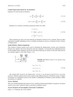
Manometry
The hydrostatic pressure variation may be employed to measure pressure differences in terms of heights
of liquid columns Ñ such devices are called manometers and are commonly used in wind tunnels and
a host of other applications and devices. Consider, for example the U-tube manometer shown in Figure
3.1.1 Þlled with liquid of speciÞc weight g, the left leg open to the atmosphere and the right to the region
whose pressure p is to be determined. In terms of the quantities shown in the Þgure, in the left leg
p0 - rgh2 = patm

(3.1.5a)

p0 - rgh1 = p

(3.1.5b)

p - patm = -rg(h1 - h2 ) = -rgd = - gd

(3.1.6)

and in the right leg

the difference being

FIGURE 3.1.1 U-tube manometer.

© 1999 by CRC Press LLC


3-4

Section 3

and determining p in terms of the height difference d = h1 Ð h2 between the levels of the ßuid in the
two legs of the manometer.

Hydrostatic Forces on Submerged Objects
We now consider the force acting on a submerged object due to the hydrostatic pressure. This is given by
F=

òò p dA = òò p × n dA = òò rgh dA + p òò dA
0

(3.1.7)

where h is the variable vertical depth of the element dA and p0 is the pressure at the surface. In turn we
consider plane and nonplanar surfaces.
Forces on Plane Surfaces
Consider the planar surface A at an angle q to a free surface shown in Figure 3.1.2. The force on one
side of the planar surface, from Equation (3.1.7), is
F = rgn

òò h dA + p An

(3.1.8)

0

A

but h = y sin q, so

òò h dA = sin qòò y dA = y Asin q = h A
c

A

c

(3.1.9)

A

where the subscript c indicates the distance measured to the centroid of the area A. Thus, the total force
(on one side) is
F = ghc A + p0 A

(3.1.10)

Thus, the magnitude of the force is independent of the angle q, and is equal to the pressure at the
centroid, ghc + p0, times the area. If we use gauge pressure, the term p0A in Equation (3.1.10) can be
dropped.
Since p is not evenly distributed over A, but varies with depth, F does not act through the centroid.
The point action of F, called the center of pressure, can be determined by considering moments in Figure
3.1.2. The moment of the hydrostatic force acting on the elementary area dA about the axis perpendicular
to the page passing through the point 0 on the free surface is
y dF = y( g y sin q dA) = g y 2 sin q dA

(3.1.11)

so if ycp denotes the distance to the center of pressure,
ycp F = g sin q

òò y

2

dA = g sin q I x

(3.1.12)

where Ix is the moment of inertia of the plane area with respect to the axis formed by the intersection
of the plane containing the planar surface and the free surface (say 0x). Dividing by F = ghcA =
g yc sin q A gives

© 1999 by CRC Press LLC


3-5

Fluid Mechanics

FIGURE 3.1.2 Hydrostatic force on a plane surface.

ycp =

Ix
yc A

(3.1.13)

By using the parallel axis theorem Ix = Ixc + Ayc2 , where Ixc is the moment of inertia with respect to an

axis parallel to 0x passing through the centroid, Equation (3.1.13) becomes
ycp = yc +

I xc
yc A

(3.1.14)

which shows that, in general, the center of pressure lies below the centroid.
Similarly, we Þnd xcp by taking moments about the y axis, speciÞcally
x cp F = g sin q

òò xy dA = g sin q I

xy

(3.1.15)

or
x cp =

I xy
yc A

(3.1.16)

where Ixy is the product of inertia with respect to the x and y axes. Again, the parallel axis theorem Ixy
= Ixyc + Axcyc, where the subscript c denotes the value at the centroid, allows Equation (3.1.16) to be written
x cp = x c +

I xyc
yc A

(3.1.17)

This completes the determination of the center of pressure (xcp, ycp). Note that if the submerged area is
symmetrical with respect to an axis passing through the centroid and parallel to either the x or y axes
that Ixyc = 0 and xcp = xc; also that as yc increases, ycp ® yc.
Centroidal moments of inertia and centroidal coordinates for some common areas are shown in Figure
3.1.3.

© 1999 by CRC Press LLC


3-6

Section 3

FIGURE 3.1.3 Centroidal moments of inertia and coordinates for some common areas.

Forces on Curved Surfaces
On a curved surface the forces on individual elements of area differ in direction so a simple summation
of them is not generally possible, and the most convenient approach to calculating the pressure force
on the surface is by separating it into its horizontal and vertical components.
A free-body diagram of the forces acting on the volume of ßuid lying above a curved surface together
with the conditions of static equilibrium of such a column leads to the results that:
1. The horizontal components of force on a curved submerged surface are equal to the forces exerted
on the planar areas formed by the projections of the curved surface onto vertical planes normal
to these components, the lines of action of these forces calculated as described earlier for planar
surfaces; and

2. The vertical component of force on a curved submerged surface is equal in magnitude to the
weight of the entire column of ßuid lying above the curved surface, and acts through the center
of mass of this volume of ßuid.
Since the three components of force, two horizontal and one vertical, calculated as above, need not meet
at a single point, there is, in general, no single resultant force. They can, however, be combined into a
single force at any arbitrary point of application together with a moment about that point.

Hydrostatic Forces in Layered Fluids
All of the above results which employ the linear hydrostatic variation of pressure are valid only for
homogeneous ßuids. If the ßuid is heterogeneous, consisting of individual layers each of constant density,
then the pressure varies linearly with a different slope in each layer and the preceding analyses must be
remedied by computing and summing the separate contributions to the forces and moments.

© 1999 by CRC Press LLC


Fluid Mechanics

3-7

Buoyancy
The same principles used above to compute hydrostatic forces can be used to calculate the net pressure
force acting on completely submerged or ßoating bodies. These laws of buoyancy, the principles of
Archimedes, are that:
1. A completely submerged body experiences a vertical upward force equal to the weight of the
displaced ßuid; and
2. A ßoating or partially submerged body displaces its own weight in the ßuid in which it ßoats
(i.e., the vertical upward force is equal to the body weight).
The line of action of the buoyancy force in both (1) and (2) passes through the centroid of the displaced
volume of ßuid; this point is called the center of buoyancy. (This point need not correspond to the center

of mass of the body, which could have nonuniform density. In the above it has been assumed that the
displaced ßuid has a constant g. If this is not the case, such as in a layered ßuid, the magnitude of the
buoyant force is still equal to the weight of the displaced ßuid, but the line of action of this force passes
through the center of gravity of the displaced volume, not the centroid.)
If a body has a weight exactly equal to that of the volume of ßuid it displaces, it is said to be neutrally
buoyant and will remain at rest at any point where it is immersed in a (homogeneous) ßuid.

Stability of Submerged and Floating Bodies
Submerged Body
A body is said to be in stable equilibrium if, when given a slight displacement from the equilibrium
position, the forces thereby created tend to restore it back to its original position. The forces acting on
a submerged body are the buoyancy force, FB, acting through the center of buoyancy, denoted by CB,
and the weight of the body, W, acting through the center of gravity denoted by CG (see Figure 3.1.4).
We see from Figure 3.1.4 that if the CB lies above the CG a rotation from the equilibrium position
creates a restoring couple which will rotate the body back to its original position Ñ thus, this is a stable
equilibrium situation. The reader will readily verify that when the CB lies below the CG, the couple
that results from a rotation from the vertical increases the displacement from the equilibrium position
Ñ thus, this is an unstable equilibrium situation.

FIGURE 3.1.4 Stability for a submerged body.

Partially Submerged Body
The stability problem is more complicated for ßoating bodies because as the body rotates the location
of the center of buoyancy may change. To determine stability in these problems requires that we determine
the location of the metacenter. This is done for a symmetric body by tilting the body through a small
angle Dq from its equilibrium position and calculating the new location of the center of buoyancy CB¢;
the point of intersection of a vertical line drawn upward from CB¢ with the line of symmetry of the
ßoating body is the metacenter, denoted by M in Figure 3.1.5, and it is independent of Dq for small
angles. If M lies above the CG of the body, we see from Figure 3.1.5 that rotation of the body leads to

© 1999 by CRC Press LLC


3-8

Section 3

FIGURE 3.1.5 Stability for a partially submerged body.

a restoring couple, whereas M lying below the CG leads to a couple which will increase the displacement.
Thus, the stability of the equilibrium depends on whether M lies above or below the CG. The directed
distance from CG to M is called the metacentric height, so equivalently the equilibrium is stable if this
vector is positive and unstable if it is negative; stability increases as the metacentric height increases.
For geometrically complex bodies, such as ships, the computation of the metacenter can be quite
complicated.

Pressure Variation in Rigid-Body Motion of a Fluid
In rigid-body motion of a òuid all the particles translate and rotate as a whole, there is no relative motion
between particles, and hence no viscous stresses since these are proportional to velocity gradients. The
equation of motion is then a balance among pressure, gravity, and the òuid acceleration, speciịcally.
ẹp = r( g - a)

(3.1.18)

where a is the uniform acceleration of the body. Equation (3.1.18) shows that the lines of constant
pressure, including a free surface if any, are perpendicular to the direction g é a. Two important
applications of this are to a òuid in uniform linear translation and rigid-body rotation. While such
problems are not, strictly speaking, òuid statics problems, their analysis and the resulting pressure
variation results are similar to those for static òuids.
Uniform Linear Acceleration

For a òuid partially ịlling a large container moving to the right with constant acceleration a = (ax, ay)
the geometry of Figure 3.1.6 shows that the magnitude of the pressure gradient in the direction n normal
to the accelerating free surface, in the direction g é a, is

(

)

2 12
dp
= rộa x2 + g + a y ự
ờở
ỷỳ
dn

(3.1.19)

and the free surface is oriented at an angle to the horizontal
ổ a ử
x
q = tan -1 ỗ
ữ
ố g + ay ứ

â 1999 by CRC Press LLC

(3.1.20)


Fluid Mechanics

3-9

FIGURE 3.1.6 A ßuid with a free surface in uniform linear acceleration.

Rigid-Body Rotation
Consider the ßuid-Þlled circular cylinder rotating uniformly with angular velocity W = Wer (Figure 3.1.7).
The only acceleration is the centripetal acceleration W ´ W ´ r) = Ð rW2 er, so Equation 3.1.18 becomes

FIGURE 3.1.7 A ßuid with a free surface in rigid-body rotation.

© 1999 by CRC Press LLC


3-10

Section 3

Ñp =

¶p
¶p
er +
e = r( g - a) = r r W 2 er - gez
¶r
¶z z

(

)

(3.1.21)

or
¶p
= rr W 2 ,
¶r

¶p
= -rg = - g
¶z

(3.1.22)

Integration of these equations leads to
p = po - g z +

1 2 2
rr W
2

(3.1.23)

where po is some reference pressure. This result shows that at any Þxed r the pressure varies hydrostatically in the vertical direction, while the constant pressure surfaces, including the free surface, are
paraboloids of revolution.

Further Information
The reader may Þnd more detail and additional information on the topics in this section in any one of
the many excellent introductory texts on ßuid mechanics, such as
White, F.M. 1994. Fluid Mechanics, 3rd ed., McGraw-Hill, New York.

Munson, B.R., Young, D.F., and Okiishi, T.H. 1994. Fundamentals of Fluid Mechanics, 2nd ed., John
Wiley & Sons, New York.

© 1999 by CRC Press LLC


3-11

Fluid Mechanics

3.2 Equations of Motion and Potential Flow
Stanley A. Berger
Integral Relations for a Control Volume
Like most physical conservation laws those governing motion of a ßuid apply to material particles or
systems of such particles. This so-called Lagrangian viewpoint is generally not as useful in practical
ßuid ßows as an analysis through Þxed (or deformable) control volumes Ñ the Eulerian viewpoint. The
relationship between these two viewpoints can be deduced from the Reynolds transport theorem, from
which we also most readily derive the governing integral and differential equations of motion.

Reynolds Transport Theorem
The extensive quantity B, a scalar, vector, or tensor, is deÞned as any property of the ßuid (e.g.,
momentum, energy) and b as the corresponding value per unit mass (the intensive value). The Reynolds
transport theorem for a moving and arbitrarily deforming control volume CV, with boundary CS (see
Figure 3.2.1), states that
d
dæ
Bsystem = ç
dt
dt çè

(

)

òòò
CV

ö
rb du÷ +
÷
ø

òò rb(V × n) dA
r

(3.2.1)

CS

where Bsystem is the total quantity of B in the system (any mass of Þxed identity), n is the outward normal
to the CS, Vr = V(r, t) Ð VCS(r, t), the velocity of the ßuid particle, V(r, t), relative to that of the CS,
VCS(r, t), and d/dt on the left-hand side is the derivative following the ßuid particles, i.e., the ßuid mass
comprising the system. The theorem states that the time rate of change of the total B in the system is
equal to the rate of change within the CV plus the net ßux of B through the CS. To distinguish between
the d/dt which appears on the two sides of Equation (3.2.1) but which have different interpretations, the
derivative on the left-hand side, following the system, is denoted by D/Dt and is called the material
derivative. This notation is used in what follows. For any function f(x, y, z, t),
Df ¶f
=
+ V × Ñf

Dt ¶t
For a CV Þxed with respect to the reference frame, Equation (3.2.1) reduces to

(

)

D
d
B
=
Dt system
dt

òòò (rb) du + òò rb(V × n) dA
CV

( fixed )

(3.2.2)

CS

(The time derivative operator in the Þrst term on the right-hand side may be moved inside the integral,
in which case it is then to be interpreted as the partial derivative ¶/¶t.)

Conservation of Mass
If we apply Equation (3.2.2) for a Þxed control volume, with Bsystem the total mass in the system, then
since conservation of mass requires that DBsystem/Dt = 0 there follows, since b = Bsystem/m = 1,

© 1999 by CRC Press LLC


3-12

Section 3

FIGURE 3.2.1 Control volume.

¶r

òòò ¶t du + òò r(V × n) dA = 0

CV
( fixed )

(3.2.3)

CS

This is the integral form of the conservation of mass law for a Þxed control volume. For a steady ßow,
Equation (3.2.3) reduces to

òò r(V × n) dA = 0

(3.2.4)

CS

whether compressible or incompressible. For an incompressible ßow, r = constant, so

òò (V × n) dA = 0

(3.2.5)

CS

whether the ßow is steady or unsteady.

Conservation of Momentum
The conservation of (linear) momentum states that

Ftotal º

å (external forces acting on the fluid system) =

æ
ö
DM
D
ç
rV du÷
º
÷
Dt
Dt ç
è system
ø

òòò

(3.2.6)

where M is the total system momentum. For an arbitrarily moving, deformable control volume it then
follows from Equation (3.2.1) with b set to V,

Ftotal =

dæ
ç
dt çè

òòò
CV

ö
rV du÷ +
÷
ø

òò rV(V × n) dA
r

(3.2.7)

CS

This expression is only valid in an inertial coordinate frame. To write the equivalent expression for a
noninertial frame we must use the relationship between the acceleration aI in an inertial frame and the
acceleration aR in a noninertial frame,

© 1999 by CRC Press LLC


3-13

Fluid Mechanics

aI = aR +

d2R
dW
+ 2W V + W (W r ) +
r
dt 2
dt

(3.2.8)

where R is the position vector of the origin of the noninertial frame with respect to that of the inertial
frame, W is the angular velocity of the noninertial frame, and r and V the position and velocity vectors
in the noninertial frame. The third term on the right-hand side of Equation (3.2.8) is the Coriolis
acceleration, and the fourth term is the centrifugal acceleration. For a noninertial frame Equation (3.2.7)
is then

Ftotal -

=

ổ
ử

ộd2R
ự
dW
D
ỗ
ữ
d
d
+
2W

V
+
W

W

r
+

r
r
u
=
r
V
u
(
)
ờ dt 2

ỳ
ữ
dt
Dt ỗ
ở
ỷ
ố system
ứ
system

ũũũ

dổ
ỗ
dt ỗố

ũũũ
CV

ũũũ

ử
rV duữ +
ữ
ứ

(3.2.9)

ũũ rV ì (V ì n) dA
r

CS

where the frame acceleration terms of Equation (3.2.8) have been brought to the left-hand side because
to an observer in the noninertial frame they act as ềapparentể body forces.
For a ịxed control volume in an inertial frame for steady òow it follows from the above that
Ftotal =

ũũ rV(V ì n) dA

(3.2.10)

CS

This expression is the basis of many control volume analyses for òuid òow problems.
The cross product of r, the position vector with respect to a convenient origin, with the momentum
Equation (3.2.6) written for an elementary particle of mass dm, noting that (dr/dt) V = 0, leads to the
integral moment of momentum equation

ồM - M

I

=

D
Dt

ũũũ r(r V ) du

(3.2.11)

system

where SM is the sum of the moments of all the external forces acting on the system about the origin of
r, and MI is the moment of the apparent body forces (see Equation (3.2.9)). The right-hand side can be
written for a control volume using the appropriate form of the Reynolds transport theorem.

Conservation of Energy
The conservation of energy law follows from the ịrst law of thermodynamics for a moving system
ổ
ử
D
ỗ
re duữ
Qầ - Wầ =
ữ
Dt ỗ
ố system
ứ

ũũũ

(3.2.12)

where Qầ is the rate at which heat is added to the system, Wầ the rate at which the system works on
its surroundings, and e is the total energy per unit mass. For a particle of mass dm the contributions to
the speciịc energy e are the internal energy u, the kinetic energy V2/2, and the potential energy, which
in the case of gravity, the only body force we shall consider, is gz, where z is the vertical displacement
opposite to the direction of gravity. (We assume no energy transfer owing to chemical reaction as well

â 1999 by CRC Press LLC


3-14

Section 3

as no magnetic or electric ịelds.) For a ịxed control volume it then follows from Equation (3.2.2) [with
b = e = u + (V2/2) + gz] that
dổ
Qầ - Wầ = ỗ
dt ỗố

ũũũ
CV

ử
1
rổ u + V 2 + gzử duữ +
ố
ứ ữ
2
ứ

ổ

ũũ rố u + 2 V
1

CS

2

+ gzử (V ì n) dA
ứ

(3.2.13)

Problem
An incompressible òuid òows through a pump at a volumetric òow rate Q. The (head) loss between
sections 1 and 2 (see Figure 3.2.2 ) is equal to brV12 / 2 (V is the average velocity at the section).
Calculate the power that must be delivered by the pump to the òuid to produce a given increase in
pressure, Dp = p2 é p1.

FIGURE 3.2.2 Pump producing pressure increase.

Solution: The principal equation needed is the energy Equation (3.2.13). The term Wầ, the rate at which
the system does work on its surroundings, for such problems has the form
Wầ = -Wầshaft +

ũũ pV ì n dA

(P.3.2.1)

CS

where Wầshaft represents the work done on the òuid by a moving shaft, such as by turbines, propellers,
fans, etc., and the second term on the right side represents the rate of working by the normal stress, the
pressure, at the boundary. For a steady òow in a control volume coincident with the physical system
boundaries and bounded at its ends by sections 1 and 2, Equation (3.2.13) reduces to (u 0),

Qầ + Wầshaft -

ổ1

ũũ pV ì n dA = ũũ ố 2 rV
CS

CS

2

+ gzử (V ì n) dA
ứ

(P.3.2.2)

Using average quantities at sections 1 and 2, and the continuity Equation (3.2.5), which reduces in this
case to
V1 A1 = V2 A2 = Q

(P.3.2.3)

We can write Equation (P.3.2.2) as
1
Qầ + Wầshaft - ( p2 - p1 ) Q = ộờ r V22 - V12 + g ( z2 - z1 )ựỳ Q
ỷ
ở2

(

â 1999 by CRC Press LLC

)

(P.3.2.4)


3-15

Fluid Mechanics

Qầ, the rate at which heat is added to the system, is here equal to é brV12 / 2, the head loss between
sections 1 and 2. Equation (P.3.2.4) then can be rewritten
2

(

)

V
1
Wầshaft = br 1 + ( Dp) Q + r V22 - V12 Q + g ( z2 - z1 ) Q
2
2
or, in terms of the given quantities,
A2 ử
brQ2
1 Q3 ổ
Wầshaft =
+ ( Dp) Q + r 2 ỗ1 - 22 ữ + g ( z2 - z1 ) Q

2
2 A2 ố
A1
A1 ứ

(P.3.2.5)

Thus, for example, if the òuid is water (r ằ 1000 kg/m3, g = 9.8 kN/m3), Q = 0.5 m3/sec, the heat
loss is 0.2rV12 / 2, and Dp = p2 é p1 = 2 105N/m2 = 200 kPa, A1 = 0.1 m2 = A2/2, (z2 é z1) = 2 m, we
ịnd, using Equation (P.3.2.5)
0.2(1000) (0.5)
1
(0.5)
+ 2 10 5 (0.5) + (1000)
Wầshaft =
(1 - 4) + 9.8 10 3 (2) (0.5)
2
(0.1)2
(0.2)2
2

(

3

)

(

)

= 5, 000 + 10, 000 - 4, 688 + 9, 800 = 20,112 Nm sec
= 20,112 W =

20,112
hp = 27 hp
745.7

Differential Relations for Fluid Motion
In the previous section the conservation laws were derived in integral form. These forms are useful in
calculating, generally using a control volume analysis, gross features of a òow. Such analyses usually
require some a priori knowledge or assumptions about the òow. In any case, an approach based on
integral conservation laws cannot be used to determine the point-by-point variation of the dependent
variables, such as velocity, pressure, temperature, etc. To do this requires the use of the differential forms
of the conservation laws, which are presented below.

Mass ConservationContinuity Equation
Applying Gaussếs theorem (the divergence theorem) to Equation (3.2.3) we obtain
ộ ảr

ự

ũũũ ờở ảt + ẹ ì (rV )ỳỷ du = 0

(3.2.14)

CV

( fixed )

which, because the control volume is arbitrary, immediately yields
ảr
+ ẹ ì (rV ) = 0
ảt

(3.2.15)

Dr
+ rẹ ì V = 0
Dt

(3.2.16)

This can also be written as

â 1999 by CRC Press LLC


3-16

Section 3

using the fact that
Dr ¶r
=
+ V × Ñr
Dt
¶t

(3.2.17)

Ñ × (rV ) = 0

(3.2.18)

Ñ×V = 0

(3.2.19)

Special cases:
1. Steady ßow [(¶/¶t) ( ) º 0]

2. Incompressible ßow (Dr/Dt º 0)

Momentum Conservation
We note Þrst, as a consequence of mass conservation for a system, that the right-hand side of Equation
(3.2.6) can be written as
æ
ö
D
DV
ç
rV du÷ º
r
du
÷
Dt ç
Dt
è system
ø system

òòò

òòò

(3.2.20)

The total force acting on the system which appears on the left-hand side of Equation (3.2.6) is the sum
of body forces Fb and surface forces Fs. The body forces are often given as forces per unit mass (e.g.,
gravity), and so can be written
Fb =

òòò rf du

(3.2.21)

system

The surface forces are represented in terms of the second-order stress tensor* s = {sij}, where sij is
deÞned as the force per unit area in the i direction on a planar element whose normal lies in the j
direction. From elementary angular momentum considerations for an inÞnitesimal volume it can be
shown that sij is a symmetric tensor, and therefore has only six independent components. The total
surface force exerted on the system by its surroundings is then
Fs =

òò s × n dA, with i - component F = òò s n
si

ij

j

dA

(3.2.22)

system
surface

The integral momentum conservation law Equation (3.2.6) can then be written

òòò r Dt

DV

system

*

du =

òòò rf du + òò s × n dA

system

(3.2.23)

system
surface

We shall assume the reader is familiar with elementary Cartesian tensor analysis and the associated subscript
notation and conventions. The reader for whom this is not true should skip the details and concentrate on the Þnal
principal results and equations given at the ends of the next few subsections.
© 1999 by CRC Press LLC


3-17

Fluid Mechanics

The application of the divergence theorem to the last term on the right-side of Equation (3.2.23) leads to

òòò r Dt

DV

du =

system

òòò rf du + òòò Ñ × s du

system

(3.2.24)

system

where Ñ á s º {¶sij/xj}. Since Equation (3.2.24) holds for any material volume, it follows that
r

DV
= rf + Ñ × s
Dt

(3.2.25)

(With the decomposition of Ftotal above, Equation (3.2.10) can be written

òòò rf du + òò s × n dA = òò rV(V × n) dA
CV

CS

(3.2.26)

CS

If r is uniform and f is a conservative body force, i.e., f = ÐÑY, where Y is the force potential, then
Equation (3.2.26), after application of the divergence theorem to the body force term, can be written

òò (-rYn + s × n) dA = òò rV(V × n) dA
CS

(3.2.27)

CS

It is in this form, involving only integrals over the surface of the control volume, that the integral form
of the momentum equation is used in control volume analyses, particularly in the case when the body

force term is absent.)

Analysis of Rate of Deformation
The principal aim of the following two subsections is to derive a relationship between the stress and the
rate of strain to be used in the momentum Equation (3.2.25). The reader less familiar with tensor notation
may skip these sections, apart from noting some of the terms and quantities deÞned therein, and proceed
directly to Equations (3.2.38) or (3.2.39).
The relative motion of two neighboring points P and Q, separated by a distance h, can be written
(using u for the local velocity)
u(Q) = u( P) + (Ñu)h
or, equivalently, writing Ñu as the sum of antisymmetric and symmetric tensors,
u(Q) = u( P) +

(

)

(

)

1
1
(Ñu) - (Ñu)* h + (Ñu) + (Ñu)* h
2
2

(3.2.28)

where Ñu = {¶ui/¶xj}, and the superscript * denotes transpose, so (Ñu)* = {¶uj/¶xi}. The second term

on the right-hand side of Equation (3.2.28) can be rewritten in terms of the vorticity, Ñ ´ u, so Equation
(3.2.28) becomes
u(Q) = u( P) +

© 1999 by CRC Press LLC

(

)

1
1
(Ñ ´ u) ´ h + (Ñu) + (Ñu)* h
2
2

(3.2.29)


3-18

Section 3

which shows that the local rate of deformation consists of a rigid-body translation, a rigid-body rotation
with angular velocity 1/2 (Ñ ´ u), and a velocity or rate of deformation. The coefÞcient of h in the last
term in Equation (3.2.29) is deÞned as the rate-of-strain tensor and is denoted by e , in subscript form

eij =

1 æ ¶ui ¶u j ö

+
2 çè ¶x j ¶xi ÷ø

(3.2.30)

From e we can deÞne a rate-of-strain central quadric, along the principal axes of which the deforming
motion consists of a pure extension or compression.

Relationship Between Forces and Rate of Deformation
We are now in a position to determine the required relationship between the stress tensor s and the
rate of deformation. Assuming that in a static ßuid the stress reduces to a (negative) hydrostatic or
thermodynamic pressure, equal in all directions, we can write
s = - pI + t or s ij = - pd ij + t ij

(3.2.31)

where t is the viscous part of the total stress and is called the deviatoric stress tensor, I is the identity
tensor, and dij is the corresponding Kronecker delta (dij = 0 if i ¹ j; dij = 1 if i = j). We make further
assumptions that (1) the ßuid exhibits no preferred directions; (2) the stress is independent of any previous
history of distortion; and (3) that the stress depends only on the local thermodynamic state and the
kinematic state of the immediate neighborhood. Precisely, we assume that t is linearly proportional to
the Þrst spatial derivatives of u, the coefÞcient of proportionality depending only on the local thermodynamic state. These assumptions and the relations below which follow from them are appropriate for
a Newtonian ßuid. Most common ßuids, such as air and water under most conditions, are Newtonian,
but there are many other ßuids, including many which arise in industrial applications, which exhibit socalled non-Newtonian properties. The study of such non-Newtonian ßuids, such as viscoelastic ßuids,
is the subject of the Þeld of rheology.
With the Newtonian ßuid assumptions above, and the symmetry of t which follows from the
symmetry of s , one can show that the viscous part t of the total stress can be written as
t = l (Ñ × u) I + 2 m e

(3.2.32)

s = - pI + l(Ñ × u) I + 2me

(3.2.33)

æ ¶u
¶u j ö
æ ¶u ö
s ij = - pd ij + l ç k ÷ d ij + mç i +
÷
è ¶x k ø
è ¶x j ¶xi ø

(3.2.34)

so the total stress for a Newtonian ßuid is

or, in subscript notation

(the Einstein summation convention is assumed here, namely, that a repeated subscript, such as in the
second term on the right-hand side above, is summed over; note also that Ñ á u = ¶uk/¶xk = ekk.) The
coefÞcient l is called the Òsecond viscosityÓ and m the Òabsolute viscosity,Ó or more commonly the
Òdynamic viscosity,Ó or simply the Òviscosity.Ó For a Newtonian ßuid l and m depend only on local
thermodynamic state, primarily on the temperature.

© 1999 by CRC Press LLC


3-19

Fluid Mechanics

We note, from Equation (3.2.34), that whereas in a ßuid at rest the pressure is an isotropic normal
stress, this is not the case for a moving ßuid, since in general s11 ¹ s22 ¹ s33. To have an analogous
quantity to p for a moving ßuid we deÞne the pressure in a moving ßuid as the negative mean normal
stress, denoted, say, by p
1
p = - s ii
3

(3.2.35)

(sii is the trace of s and an invariant of s , independent of the orientation of the axes). From Equation
(3.2.34)
1
2
p = - s ii = p - æ l + mö Ñ × u
è
3
3 ø

(3.2.36)

For an incompressible ßuid Ñ á u = 0 and hence p º p. The quantity (l + 2/3m) is called the bulk
viscosity. If one assumes that the deviatoric stress tensor tij makes no contribution to the mean normal
stress, it follows that l + 2/3m = 0, so again p = p. This condition, l = Ð2/3m, is called the Stokes
assumption or hypothesis. If neither the incompressibility nor the Stokes assumptions are made, the
difference between p and p is usually still negligibly small because (l + 2/3m) Ñ á u << p in most ßuid
ßow problems. If the Stokes hypothesis is made, as is often the case in ßuid mechanics, Equation (3.2.34)
becomes

1
s ij = - pd ij + 2mæ eij - ekk d ij ö
è
ø
3

(3.2.37)

The Navier–Stokes Equations
Substitution of Equation (3.2.33) into (3.2.25), since Ñ á (fI ) = Ñf, for any scalar function f, yields
(replacing u in Equation (3.2.33) by V)
r

( )

DV
= rf - Ñp + Ñ(lÑ × V ) + Ñ × 2me
Dt

(3.2.38)

These equations are the NavierÐStokes equations (although the name is as often given to the full set of
governing conservation equations). With the Stokes assumption (l = Ð2/3m), Equation (3.2.38) becomes
r

1
DV
ù
é
= rf - Ñp + Ñ × ê2mæ e - ekk I ö ú

øû
3
Dt
ë è

(3.2.39)

If the Eulerian frame is not an inertial frame, then one must use the transformation to an inertial frame
either using Equation (3.2.8) or the ÒapparentÓ body force formulation, Equation (3.2.9).

Energy Conservation — The Mechanical and Thermal Energy Equations
In deriving the differential form of the energy equation we begin by assuming that heat enters or leaves
the material or control volume by heat conduction across the boundaries, the heat ßux per unit area
being q. It then follows that
QÇ = -

© 1999 by CRC Press LLC

òò q × n dA = -òòò Ñ × q du

(3.2.40)


3-20

Section 3

The work-rate term Wầ can be decomposed into the rate of work done against body forces, given by

é

ũũũ rf ì V du

(3.2.41)

and the rate of work done against surface stresses, given by
-

ũũ V ì (s n) dA

(3.2.42)

system
surface

Substitution of these expressions for Qầ and Wầ into Equation (3.2.12), use of the divergence theorem,
and conservation of mass lead to
r

( )

1
Dổ
u + V 2 ử = -ẹ ì q + rf ì V + ẹ ì V s
ố
2 ứ
Dt

(3.2.43)

(note that a potential energy term is no longer included in e, the total speciịc energy, as it is accounted
for by the body force rate-of-working term rf ỏ V).
Equation (3.2.43) is the total energy equation showing how the energy changes as a result of working
by the body and surface forces and heat transfer. It is often useful to have a purely thermal energy
equation. This is obtained by subtracting from Equation (3.2.43) the dot product of V with the momentum
Equation (3.2.25), after expanding the last term in Equation (3.2.43), resulting in
r

Du ảVi
=
s - ẹìq
Dt ảx j ij

(3.2.44)

With sij = épdij + tij, and the use of the continuity equation in the form of Equation (3.2.16), the ịrst
term on the right-hand side of Equation (3.2.44) may be written
ổ pử
Dỗ ữ
ảVi
ố r ứ Dp
s = -r
+
+F
Dt
Dt
ảx j ij

(3.2.45)

where F is the rate of dissipation of mechanical energy per unit mass due to viscosity, and is given by
F

2
ảVi
1 2ử
1
t ij = 2mổ eij eij - ekk
= 2mổ eij - ekk d ij ử
ố
ố
ứ
ảx j
3 ứ
3

(3.2.46)

With the introduction of Equation (3.2.45), Equation (3.2.44) becomes
r

De
= - pẹ ì V + F - ẹ ì q
Dt

(3.2.47)

Dh Dp
=
+ F - ẹìq

Dt
Dt

(3.2.48)

or
r

â 1999 by CRC Press LLC


3-21

Fluid Mechanics

where h = e + (p/r) is the speciÞc enthalpy. Unlike the other terms on the right-hand side of Equation
(3.2.47), which can be negative or positive, F is always nonnegative and represents the increase in
internal energy (or enthalpy) owing to irreversible degradation of mechanical energy. Finally, from
elementary thermodynamic considerations
Dh
DS 1 Dp
=T
+
Dt
Dt r Dt
where S is the entropy, so Equation (3.2.48) can be written
rT

DS
= F - Ñ×q

Dt

(3.2.49)

If the heat conduction is assumed to obey the Fourier heat conduction law, so q = Ð kÑT, where k is the
thermal conductivity, then in all of the above equations
- Ñ × q = Ñ × (kÑT ) = kÑ 2 T

(3.2.50)

the last of these equalities holding only if k = constant.
In the event the thermodynamic quantities vary little, the coefÞcients of the constitutive relations for
s and q may be taken to be constant and the above equations simpliÞed accordingly.
We note also that if the ßow is incompressible, then the mass conservation, or continuity, equation
simpliÞes to
Ñ×V = 0

(3.2.51)

and the momentum Equation (3.2.38) to
r

DV
= rf - Ñp + mÑ 2 V
Dt

(3.2.52)

where Ñ2 is the Laplacian operator. The small temperature changes, compatible with the incompressibility
assumption, are then determined, for a perfect gas with constant k and speciÞc heats, by the energy

equation rewritten for the temperature, in the form
rcv

DT
= kÑ 2 T + F
Dt

(3.2.53)

Boundary Conditions
The appropriate boundary conditions to be applied at the boundary of a ßuid in contact with another
medium depends on the nature of this other medium Ñ solid, liquid, or gas. We discuss a few of the
more important cases here in turn:
1. At a solid surface: V and T are continuous. Contained in this boundary condition is the Òno-slipÓ
condition, namely, that the tangential velocity of the ßuid in contact with the boundary of the
solid is equal to that of the boundary. For an inviscid ßuid the no-slip condition does not apply,
and only the normal component of velocity is continuous. If the wall is permeable, the tangential
velocity is continuous and the normal velocity is arbitrary; the temperature boundary condition
for this case depends on the nature of the injection or suction at the wall.
© 1999 by CRC Press LLC


3-22

Section 3

2. At a liquid/gas interface: For such cases the appropriate boundary conditions depend on what
can be assumed about the gas the liquid is in contact with. In the classical liquid free-surface
problem, the gas, generally atmospheric air, can be ignored and the necessary boundary conditions
are that (a) the normal velocity in the liquid at the interface is equal to the normal velocity of the

interface and (b) the pressure in the liquid at the interface exceeds the atmospheric pressure by
an amount equal to
æ 1
1ö
Dp = pliquid - patm = sç + ÷
R
R
è 1
2ø

(3.2.54)

where R1 and R2 are the radii of curvature of the intercepts of the interface by two orthogonal
planes containing the vertical axis. If the gas is a vapor which undergoes nonnegligible interaction
and exchanges with the liquid in contact with it, the boundary conditions are more complex. Then,
in addition to the above conditions on normal velocity and pressure, the shear stress (momentum
ßux) and heat ßux must be continuous as well.
For interfaces in general the boundary conditions are derived from continuity conditions for each
ÒtransportableÓ quantity, namely continuity of the appropriate intensity across the interface and continuity
of the normal component of the ßux vector. Fluid momentum and heat are two such transportable
quantities, the associated intensities are velocity and temperature, and the associated ßux vectors are
stress and heat ßux. (The reader should be aware of circumstances where these simple criteria do not
apply, for example, the velocity slip and temperature jump for a rareÞed gas in contact with a solid
surface.)

Vorticity in Incompressible Flow
With m = constant, r = constant, and f = Ðg = Ðgk the momentum equation reduces to the form (see
Equation (3.2.52))
r

DV
= -Ñp - rg k + mÑ 2 V
Dt

(3.2.55)

With the vector identities
æ V2 ö
÷ - V ´ (Ñ ´ V )
è 2 ø

(V × Ñ)V = Ñç

(3.2.56)

and
Ñ 2 V = Ñ(Ñ × V ) - Ñ ´ (Ñ ´ V )

(3.2.57)

z º Ñ´V

(3.2.58)

and deÞning the vorticity

Equation (3.2.55) can be written, noting that for incompressible ßow Ñ á V = 0,
r

© 1999 by CRC Press LLC

1
¶V
+ Ñæ p + rV 2 + rgzö = rV ´ z - mÑ ´ z
è
ø
2
¶t

(3.2.59)


3-23

Fluid Mechanics

The ßow is said to be irrotational if
z º Ñ´V = 0

(3.2.60)

from which it follows that a velocity potential F can be deÞned
V = ÑF

(3.2.61)

Setting z = 0 in Equation (3.2.59), using Equation (3.2.61), and then integrating with respect to all the
spatial variables, leads to
r

1
¶F æ
+ p + rV 2 + rgzö = F(t )
è
ø
2
¶t

(3.2.62)

(the arbitrary function F(t) introduced by the integration can either be absorbed in F, or is determined
by the boundary conditions). Equation (3.2.62) is the unsteady Bernoulli equation for irrotational,
incompressible ßow. (Irrotational ßows are always potential ßows, even if the ßow is compressible.
Because the viscous term in Equation (3.2.59) vanishes identically for z = 0, it would appear that the
above Bernoulli equation is valid even for viscous ßow. Potential solutions of hydrodynamics are in fact
exact solutions of the full NavierÐStokes equations. Such solutions, however, are not valid near solid
boundaries or bodies because the no-slip condition generates vorticity and causes nonzero z; the potential
ßow solution is invalid in all those parts of the ßow Þeld that have been ÒcontaminatedÓ by the spread
of the vorticity by convection and diffusion. See below.)
The curl of Equation (3.2.59), noting that the curl of any gradient is zero, leads to
r

¶z
= rÑ ´ (V ´ z) - mÑ ´ Ñ ´ z
¶t

(3.2.63)

but
Ñ 2z = Ñ(Ñ × z) - Ñ ´ Ñ ´ z

= -Ñ ´ Ñ ´ z

(3.2.64)

since div curl ( ) º 0, and therefore also
Ñ ´ (V ´ z) º z(ÑV ) + VÑ × z - VÑz - zÑ × V

(3.2.65)

= z(ÑV ) - VÑz

(3.2.66)

Dz
= (z × Ñ)V + nÑ 2z
Dt

(3.2.67)

Equation (3.2.63) can then be written

where n = m/r is the kinematic viscosity. Equation (3.2.67) is the vorticity equation for incompressible
ßow. The Þrst term on the right, an inviscid term, increases the vorticity by vortex stretching. In inviscid,
two-dimensional ßow both terms on the right-hand side of Equation (3.2.67) vanish, and the equation
reduces to Dz/Dt = 0, from which it follows that the vorticity of a ßuid particle remains constant as it
moves. This is HelmholtzÕs theorem. As a consequence it also follows that if z = 0 initially, z º 0 always;
© 1999 by CRC Press LLC


3-24

Section 3

i.e., initially irrotational ßows remain irrotational (for inviscid ßow). Similarly, it can be proved that
DG/Dt = 0; i.e., the circulation around a material closed circuit remains constant, which is KelvinÕs
theorem.
If n ¹ 0, Equation (3.2.67) shows that the vorticity generated, say, at solid boundaries, diffuses and
stretches as it is convected.
We also note that for steady ßow the Bernoulli equation reduces to
p+

1 2
rV + rgz = constant
2

(3.2.68)

valid for steady, irrotational, incompressible ßow.

Stream Function
For two-dimensional ßows the continuity equation, e.g., for plane, incompressible ßows (V = (u, n))
¶u ¶n
+
=0
¶x ¶y

(3.2.69)

can be identically satisÞed by introducing a stream function y, deÞned by
u=

¶y
,
¶y

n=-

¶y
¶x

(3.2.70)

Physically y is a measure of the ßow between streamlines. (Stream functions can be similarly deÞned
to satisfy identically the continuity equations for incompressible cylindrical and spherical axisymmetric
ßows; and for these ßows, as well as the above planar ßow, also when they are compressible, but only
then if they are steady.) Continuing with the planar case, we note that in such ßows there is only a single
nonzero component of vorticity, given by
æ
¶n ¶u ö
z = (0, 0, z z ) = ç 0, 0,
- ÷
¶x ¶y ø
è

(3.2.71)

With Equation (3.2.70)
zz = -

¶2 y ¶2 y

- 2 = -Ñ 2 y
¶x 2
¶y

(3.2.72)

For this two-dimensional ßow Equation (3.2.67) reduces to
æ ¶ 2z
¶z z
¶z
¶z
¶ 2z z ö
+ u z + n z = nç 2z +
¶t
¶x
¶y
¶y 2 ÷ø
è ¶x

(3.2.73)

Substitution of Equation (3.2.72) into Equation (3.2.73) yields an equation for the stream function

(

¶ Ñ2 y

© 1999 by CRC Press LLC

¶t

) + ¶y ¶(Ñ y ) - ¶y
2

¶y

¶x

¶
Ñ 2 y = nÑ 4 y
¶x ¶y

(

)

(3.2.74)