Foundation mathematics for the physical sciences
Bạn đang xem bản rút gọn của tài liệu. Xem và tải ngay bản đầy đủ của tài liệu tại đây (5.07 MB, 737 trang )
This page intentionally left blank
Foundation Mathematics for the Physical Sciences
This tutorial-style textbook develops the basic mathematical tools needed by first- and secondyear undergraduates to solve problems in the physical sciences. Students gain hands-on experience
through hundreds of worked examples, end-of-section exercises, self-test questions and homework
problems.
Each chapter includes a summary of the main results, definitions and formulae. Over 270 worked
examples show how to put the tools into practice. Around 170 self-test questions in the footnotes
and 300 end-of-section exercises give students an instant check of their understanding. More than
450 end-of-chapter problems allow students to put what they have just learned into practice.
Hints and outline answers to the odd-numbered problems are given at the end of each chapter.
Complete solutions to these problems can be found in the accompanying Student Solution Manual.
Fully worked solutions to all the problems, password-protected for instructors, are available at
www.cambridge.org/foundation.
K . F . R i l e y read mathematics at the University of Cambridge and proceeded to a Ph.D. there
in theoretical and experimental nuclear physics. He became a Research Associate in elementary
particle physics at Brookhaven, and then, having taken up a lectureship at the Cavendish Laboratory,
Cambridge, continued this research at the Rutherford Laboratory and Stanford; in particular he was
involved in the experimental discovery of a number of the early baryonic resonances. As well
as having been Senior Tutor at Clare College, where he has taught physics and mathematics for
over 40 years, he has served on many committees concerned with the teaching and examining of
these subjects at all levels of tertiary and undergraduate education. He is also one of the authors of
200 Puzzling Physics Problems (Cambridge University Press, 2001).
M . P . H o b s o n read natural sciences at the University of Cambridge, specialising in theoretical
physics, and remained at the Cavendish Laboratory to complete a Ph.D. in the physics of star
formation. As a Research Fellow at Trinity Hall, Cambridge, and subsequently an Advanced Fellow
of the Particle Physics and Astronomy Research Council, he developed an interest in cosmology, and
in particular in the study of fluctuations in the cosmic microwave background. He was involved in
the first detection of these fluctuations using a ground-based interferometer. Currently a University
Reader at the Cavendish Laboratory, his research interests include both theoretical and observational
aspects of cosmology, and he is the principal author of General Relativity: An Introduction for
Physicists (Cambridge University Press, 2006). He is also a Director of Studies in Natural Sciences
at Trinity Hall and enjoys an active role in the teaching of undergraduate physics and mathematics.
Foundation Mathematics
for the Physical Sciences
K. F. RILEY
University of Cambridge
M. P. HOBSON
University of Cambridge
cambridge university press
Cambridge, New York, Melbourne, Madrid, Cape Town, Singapore,
S˜ao Paulo, Delhi, Dubai, Tokyo, Mexico City
Cambridge University Press
The Edinburgh Building, Cambridge CB2 8RU, UK
Published in the United States of America by Cambridge University Press, New York
www.cambridge.org
Information on this title: www.cambridge.org/9780521192736
C
K. Riley and M. Hobson 2011
This publication is in copyright. Subject to statutory exception
and to the provisions of relevant collective licensing agreements,
no reproduction of any part may take place without the written
permission of Cambridge University Press.
First published 2011
Printed in the United Kingdom at the University Press, Cambridge
A catalogue record for this publication is available from the British Library
Library of Congress Cataloguing in Publication data
Riley, K. F. (Kenneth Franklin), 1936–
Foundation mathematics for the physical sciences : a tutorial guide / K. F. Riley, M. P. Hobson.
p. cm.
Includes index.
ISBN 978-0-521-19273-6
1. Mathematics. I. Hobson, M. P. (Michael Paul), 1967– II. Title.
QA37.3.R56 2011
510 – dc22
2010041510
ISBN 978-0-521-19273-6 Hardback
Additional resources for this publication: www.cambridge.org/foundation
Cambridge University Press has no responsibility for the persistence or
accuracy of URLs for external or third-party internet websites referred to
in this publication, and does not guarantee that any content on such
websites is, or will remain, accurate or appropriate.
Contents
Preface
1
Arithmetic and geometry
1.1
1.2
1.3
1.4
1.5
1.6
2
3
v
Powers
Exponential and logarithmic functions
Physical dimensions
The binomial expansion
Trigonometric identities
Inequalities
Summary
Problems
Hints and answers
page xi
1
1
7
15
20
24
32
40
42
49
Preliminary algebra
52
2.1
2.2
2.3
2.4
53
64
74
84
91
93
99
Polynomials and polynomial equations
Coordinate geometry
Partial fractions
Some particular methods of proof
Summary
Problems
Hints and answers
Differential calculus
102
3.1
3.2
3.3
3.4
3.5
3.6
102
112
114
116
120
124
133
134
138
Differentiation
Leibnitz’s theorem
Special points of a function
Curvature of a function
Theorems of differentiation
Graphs
Summary
Problems
Hints and answers
vi
Contents
4
5
6
7
Integral calculus
141
4.1
4.2
4.3
4.4
4.5
4.6
4.7
4.8
141
146
152
155
156
159
160
161
168
170
173
Integration
Integration methods
Integration by parts
Reduction formulae
Infinite and improper integrals
Integration in plane polar coordinates
Integral inequalities
Applications of integration
Summary
Problems
Hints and answers
Complex numbers and hyperbolic functions
174
5.1
5.2
5.3
5.4
5.5
5.6
5.7
174
176
185
189
194
196
197
205
206
211
The need for complex numbers
Manipulation of complex numbers
Polar representation of complex numbers
De Moivre’s theorem
Complex logarithms and complex powers
Applications to differentiation and integration
Hyperbolic functions
Summary
Problems
Hints and answers
Series and limits
213
6.1
6.2
6.3
6.4
6.5
6.6
6.7
213
215
224
232
233
238
244
248
250
257
Series
Summation of series
Convergence of infinite series
Operations with series
Power series
Taylor series
Evaluation of limits
Summary
Problems
Hints and answers
Partial differentiation
259
7.1
7.2
7.3
7.4
259
261
264
266
Definition of the partial derivative
The total differential and total derivative
Exact and inexact differentials
Useful theorems of partial differentiation
vii
Contents
7.5
7.6
7.7
7.8
7.9
7.10
7.11
7.12
8
9
10
The chain rule
Change of variables
Taylor’s theorem for many-variable functions
Stationary values of two-variable functions
Stationary values under constraints
Envelopes
Thermodynamic relations
Differentiation of integrals
Summary
Problems
Hints and answers
267
268
270
272
276
282
285
288
290
292
299
Multiple integrals
301
8.1
8.2
8.3
301
305
315
324
325
329
Double integrals
Applications of multiple integrals
Change of variables in multiple integrals
Summary
Problems
Hints and answers
Vector algebra
331
9.1
9.2
9.3
9.4
9.5
9.6
9.7
9.8
331
332
336
339
346
348
353
357
359
361
368
Scalars and vectors
Addition, subtraction and multiplication of vectors
Basis vectors, components and magnitudes
Multiplication of two vectors
Triple products
Equations of lines, planes and spheres
Using vectors to find distances
Reciprocal vectors
Summary
Problems
Hints and answers
Matrices and vector spaces
369
10.1
10.2
10.3
10.4
10.5
10.6
370
374
376
377
383
385
Vector spaces
Linear operators
Matrices
Basic matrix algebra
The transpose and conjugates of a matrix
The trace of a matrix
viii
Contents
10.7
10.8
10.9
10.10
10.11
10.12
10.13
10.14
10.15
10.16
10.17
11
12
The determinant of a matrix
The inverse of a matrix
The rank of a matrix
Simultaneous linear equations
Special types of square matrix
Eigenvectors and eigenvalues
Determination of eigenvalues and eigenvectors
Change of basis and similarity transformations
Diagonalisation of matrices
Quadratic and Hermitian forms
The summation convention
Summary
Problems
Hints and answers
386
392
395
397
408
412
418
421
424
427
432
433
437
445
Vector calculus
448
11.1
11.2
11.3
11.4
11.5
11.6
11.7
11.8
11.9
448
453
454
455
458
458
465
469
476
482
483
490
Differentiation of vectors
Integration of vectors
Vector functions of several arguments
Surfaces
Scalar and vector fields
Vector operators
Vector operator formulae
Cylindrical and spherical polar coordinates
General curvilinear coordinates
Summary
Problems
Hints and answers
Line, surface and volume integrals
491
12.1
12.2
12.3
12.4
12.5
12.6
12.7
12.8
12.9
491
497
498
502
504
511
513
517
523
527
528
534
Line integrals
Connectivity of regions
Green’s theorem in a plane
Conservative fields and potentials
Surface integrals
Volume integrals
Integral forms for grad, div and curl
Divergence theorem and related theorems
Stokes’ theorem and related theorems
Summary
Problems
Hints and answers
ix
Contents
13
14
15
Laplace transforms
536
13.1
13.2
13.3
13.4
537
541
544
546
549
550
552
Laplace transforms
The Dirac δ-function and Heaviside step function
Laplace transforms of derivatives and integrals
Other properties of Laplace transforms
Summary
Problems
Hints and answers
Ordinary differential equations
554
14.1
14.2
14.3
14.4
14.5
14.6
555
557
565
569
572
579
585
587
595
General form of solution
First-degree first-order equations
Higher degree first-order equations
Higher order linear ODEs
Linear equations with constant coefficients
Linear recurrence relations
Summary
Problems
Hints and answers
Elementary probability
597
15.1
15.2
15.3
15.4
15.5
15.6
15.7
15.8
15.9
597
602
612
618
623
628
632
643
655
661
664
670
Venn diagrams
Probability
Permutations and combinations
Random variables and distributions
Properties of distributions
Functions of random variables
Important discrete distributions
Important continuous distributions
Joint distributions
Summary
Problems
Hints and answers
A
The base for natural logarithms
673
B
Sinusoidal definitions
676
C
Leibnitz’s theorem
679
x
Contents
D
Summation convention
681
E
Physical constants
684
F
Footnote answers
685
Index
706
Preface
Since Mathematical Methods for Physics and Engineering by Riley, Hobson and Bence
(Cambridge: Cambridge University Press, 1998), hereafter denoted by MMPE, was first
published, the range of material it covers has increased with each subsequent edition (2002
and 2006). Most of the additions have been in the form of introductory material covering
polynomial equations, partial fractions, binomial expansions, coordinate geometry and
a variety of basic methods of proof, though the third edition of MMPE also extended
the range, but not the general level, of the areas to which the methods developed in the
book could be applied. Recent feedback suggests that still further adjustments would be
beneficial. In so far as content is concerned, the inclusion of some additional introductory
material such as powers, logarithms, the sinusoidal and exponential functions, inequalities
and the handling of physical dimensions, would make the starting level of the book better
match that of some of its readers.
To incorporate these changes, and others aimed at increasing the user-friendliness of the
text, into the current third edition of MMPE would inevitably produce a text that would be
too ponderous for many students, to say nothing of the problems the physical production
and transportation of such a large volume would entail.
For these reasons, we present under the current title, Foundation Mathematics for the
Physical Sciences, an alternative edition of MMPE, one that focuses on the earlier part
of a putative extended third edition. It omits those topics that truly are ‘methods’ and
concentrates on the ‘mathematical tools’ that are used in more advanced texts to build up
those methods. The emphasis is very much on developing the basic mathematical concepts
that a physical scientist needs, before he or she can narrow their focus onto methods that
are particularly appropriate to their chosen field.
One aspect that has remained constant throughout the three editions of MMPE is the
general style of presentation of a topic – a qualitative introduction, physically based
wherever possible, followed by a more formal presentation or proof, and finished with
one or two full-worked examples. This format has been well received by reviewers, and
there is no reason to depart from its basic structure.
In terms of style, many physical science students appear to be more comfortable with
presentations that contain significant amounts of explanation or comment in words, rather
than with a series of mathematical equations the last line of which implies ‘job done’. We
have made changes that move the text in this direction. As is explained below, we also
feel that if some of the advantages of small-group face-to-face teaching could be reflected
in the written text, many students would find it beneficial.
In keeping with the intention of presenting a more ‘gentle’ introduction to universitylevel mathematics for the physical sciences, we have made use of a modest number of
appendices. These contain the more formal mathematical developments associated with
xi
xii
Preface
the material introduced in the early chapters, and, in particular, with that discussed in the
introductory chapter on arithmetic and geometry. They can be studied at the points in the
main text where references are made to them, or deferred until a greater mathematical
fluency has been acquired.
As indicated above, one of the advantages of an oral approach to teaching, apparent to
some extent in the lecture situation, and certainly in what are usually known as tutorials,1
is the opportunity to follow the exposition of any particular point with an immediate
short, but probing, question that helps to establish whether or not the student has grasped
that point. This facility is not normally available when instruction is through a written
medium, without having available at least the equipment necessary to access the contents
of a storage disc.
In this book we have tried to go some way towards remedying this by making a nonstandard use of footnotes. Some footnotes are used in traditional ways, to add a comment or
a pertinent but not essential piece of additional information, to clarify a point by restating
it in slightly different terms, or to make reference to another part of the text or an external
source. However, about half of the more than 300 footnotes in this book contain a question
for the reader to answer or an instruction for them to follow; neither will call for a lengthy
response, but in both cases an understanding of the associated material in the text will be
required. This parallels the sort of follow-up a student might have to supply orally in a
small-group tutorial, after a particular aspect of their written work has been discussed.
Naturally, students should attempt to respond to footnote questions using the skills and
knowledge they have acquired, re-reading the relevant text if necessary, but if they are
unsure of their answer, or wish to feel the satisfaction of having their correct response
confirmed, they can consult the specimen answers given in Appendix F. Equally, footnotes
in the form of observations will have served their purpose when students are consistently
able to say to themselves ‘I didn’t need that comment – I had already spotted and checked
that particular point’.
There are two further features of the present volume that did not appear in MMPE.
The first of these is that a small set of exercises has been included at the end of each
section. The questions posed are straightforward and designed to test whether the student
has understood the concepts and procedures described in that section. The questions are
not intended as ‘drill exercises’, with repeated use of the same procedure on marginally
different sets of data; each concept is examined only once or twice within the set. There
are, nevertheless, a total of more than 300 such exercises. The more demanding questions,
and in particular those requiring the synthesis of several ideas from a chapter, are those
that appear under the heading of ‘Problems’ at the end of that chapter; there are more than
450 of these.
The second new feature is the inclusion at the end of each chapter, just before the
problems begin, of a summary of the main results of that chapter. For some areas, this
takes the form of a tabulation of the various case types that may arise in the context of
the chapter; this should help the student to see the parallels between situations which
in the main text are presented as a consecutive series of often quite lengthy pieces of
mathematical development. It should be said that in such a summary it is not possible to
••••••••••••••••••••••••••••••••••••••••••••••••••••••••••••••••••••••••••••••••••••••••••••••••••••••••••••••••
1 But in Cambridge are called ‘supervisions’!
xiii
Preface
state every detailed condition attached to each result, and the reader should consider the
summaries as reminders and formulae providers, rather than as teaching text; that is the
job of the main text and its footnotes. Fortunately, in this volume, occasions on which
subtle conditions have to be imposed upon a result are rare.
Finally, we note, for the record, that the format and numbering of the problems associated with the various chapters have not been changed significantly from those in MMPE,
though naturally only problems related to included topics are retained. This means that
abbreviated solutions to all odd-numbered problems can be found in this text. Fully worked
solutions to the same problems are available in the companion volume Student Solution
Manual for Foundation Mathematics for the Physical Sciences; most of them, except for
those in the first chapter, can also be found in the Student Solution Manual for MMPE.
Fully worked solutions to all problems, both odd- and even-numbered, are available to
accredited instructors on the password-protected website www.cambridge.org/foundation.
Instructors wishing to have access to the website should contact
for registration details.
1
Arithmetic and geometry
The first two chapters of this book review the basic arithmetic, algebra and geometry of
which a working knowledge is presumed in the rest of the text; many students will have
at least some familiarity with much, if not all, of it. However, the considerable choice
now available in what is to be studied for secondary-education examination purposes
means that none of it can be taken for granted. The reader may make a preliminary
assessment of which areas need further study or revision by first attempting the
problems at the ends of the chapters. Unlike the problems associated with all other
chapters, those for the first two are divided into named sections and each problem deals
almost exclusively with a single topic.
This opening chapter explains the basic definitions and uses associated with some
of the most common mathematical procedures and tools; these are the components
from which the mathematical methods developed in more advanced texts are built. So
as to keep the explanations as free from detailed mathematical working as possible –
and, in some cases, because results from later chapters have to be anticipated – some
justifications and proofs have been placed in appendices. The reader who chooses to
omit them on a first reading should return to them after the appropriate material has
been studied.
The main areas covered in this first chapter are powers and logarithms, inequalities,
sinusoidal functions, and trigonometric identities. There is also an important section on
the role played by dimensions in the description of physical systems. Topics that are
wholly or mainly concerned with algebraic methods have been placed in the second
chapter. It contains sections on polynomial equations, the related topic of partial
fractions, and some coordinate geometry; the general topic of curve sketching is
deferred until methods for locating maxima and minima have been developed in
Chapter 3. An introduction to the notions of proof by induction or contradiction is
included in Chapter 2, as the examples used to illustrate it are almost entirely algebraic
in nature. The same is true of a discussion of the necessary and sufficient conditions for
two mathematical statements to be equivalent.
1.1
Powers
• • • • • • • • • • • • • • • • • • • • • • • • • • • • • • • • • • • • • • • • • • • • • • • • • • • • • • • • • • • • • • • • •
If we multiply together n factors each equal to a, we call the result the nth power of a
and write it as a n . The quantity n, a positive integer in this definition, is called the index
or exponent.
1
2
Arithmetic and geometry
The algebraic rules for combining different powers of the same quantity, i.e. combining
expressions all of the form a n , but with different exponents in general, are summarised by
the four equations
pa n ± qa n = (p ± q)a n ,
(1.1)
a ×a =a
m+n
,
(1.2)
a ÷a =a
m−n
,
(1.3)
m
m
n
n
(a ) = a
m n
mn
= (a )
n m
.
(1.4)
To these can be added the rules for multiplying and dividing two powers that contain the
same exponent:
a n × bn = (ab)n ,
a n
a n ÷ bn =
.
b
(1.5)
(1.6)
The multiplication of powers is both commutative and associative. Since these terms
are relevant to characterising nearly all mathematical operations, and appear many times
in the remainder of this book, we give here a brief discussion of them.
Commutativity
An operation, denoted by say, that acts upon two objects x and y that belong to some
particular class of objects, and so produces a result x y, is said to be commutative if
x y = y x for all pairs of objects in the class; loosely speaking, it does not matter
in which order the two objects appear. As examples, for real numbers, addition (x + y =
y + x) and multiplication (x × y = y × x) are commutative, but subtraction and division
are not; the latter two fail to be commutative because x − y = y − x and x/y = y/x.
The same is true with regard to combining powers: when stands for multiplication
and x and y are a m and a n , then, since a m × a n = a n × a m , the operation of multiplication
is commutative; but, when stands for division and x and y are as before, the operation
is non-commutative because a m ÷ a n = a n ÷ a m . It might be added that not all forms of
multiplication are commutative; for example, if x and y are matrices A and B, then, in
general, AB and BA are not equal (see Chapter 10).
Associativity
Using the notation of the previous two paragraphs, the operation is said to be associative
if (x y) z = x (y z) for all triples of objects in the class; here the parentheses
indicate that the operations enclosed by them are the first to be carried out within each
grouping. Again, as simple examples, for real numbers, addition [(x + y) + z = x + (y +
z)] and multiplication [(x × y) × z = x × (y × z)] are associative, but subtraction and
division are not. Subtraction fails to be associative because (x − y) − z = x − (y − z),
i.e. x − y − z = x − y + z; division fails in a similar way.
3
1.1 Powers
Corresponding results apply to the operations of combining powers. In summary, the
multiplication of powers is both commutative and associative; the division of them is
neither.1
Given the rules set out above for combining powers, and the fact that any non-zero
value divided by itself must yield unity, we must have, on setting n = m in (1.3), that
1 = a m ÷ a m = a m−m = a 0 .
Thus, for any a = 0,
a 0 = 1.
(1.7)
The case in which a = 0 is discussed later, when logarithms are considered.
Result (1.7) has already taken us away from our original construction of a power, as
the notion of multiplying no factors of a together and obtaining unity is not altogether
intuitive; rather we must consider the process of forming a n as one of multiplying unity n
times by a factor of a.
Another consequence of result (1.3), taken together with deduction (1.7), can now be
found by setting m = 0 in (1.3). Doing this shows that, for a = 0,
1
= a 0 ÷ a n = a 0−n = a −n .
an
(1.8)
In words, the reciprocal of a n is a −n . The analogy with the construction in the previous
paragraph is that a −n is formed by dividing unity n times by a factor of a.
Rule (1.4) allows us to assign a meaning to a n when n is a general rational number,
i.e. n can be written as n = p/q where p and q are integers; n itself is not necessarily an
integer. In particular, if we take n to have the form n = 1/m, where m is an integer, then
the second equality in (1.4) reads
a = a 1 = (a 1/m )m .
(1.9)
This shows that the quantity a 1/m when raised to the mth power produces the quantity a.
This, in turn, implies that a 1/m must be interpreted as the mth root of a, otherwise denoted
√
by m a. With this identification, the first equality in (1.4) expresses the compatible result
that the mth root of a m is a.
For more general values of p and q, we have that
(a 1/q )p = a p/q = (a p )1/q ,
(1.10)
which states that the pth power of the qth root of a is equal to the qth root of the pth
power of a.
It should be noted that, so long as only real quantities are allowed, a must be confined
to positive values when taking roots in this way; the need for this will be clear from
considering the case of a negative and m an even integer. It is possible to find a valid
answer for a 1/m with a negative if m is an odd integer (or, more generally, if the q in
•••••••••••••••••••••••••••••••••••••••••••••••••••••••••••••••••••••••••••••••••••••••••••••••••••••••
1 Consider for each
√ of the following operations whether it is commutative and/or associative: (i) a
(ii) a b = + a 2 + b2 , (iii) a b = a b ; a and b are real positive numbers.
b = a 2 + b2 ,
4
Arithmetic and geometry
n = p/q is an odd integer), as is shown by the calculation
1
− 27
−4/3
= (−1)−4/3
=
1 4
−1
3 4
1
1 −4/3
27
= (−1)−4
1 −4
3
= 1 × 81 = 81.
However, both a and p/q could be more general expressions whose signs and values are
not fixed, and great care is needed when using anything other than explicit numerical
values.
Having established a meaning for a m when m is either an integer or a rational fraction,
we would also wish to attach a mathematical meaning to it when m is not confined to either
of these classes, but is any real number. Obviously, any general m that is expressed to a
finite number of decimal places could be considered formally, but very inconveniently, as
a rational fraction;
however, there are infinitely many numbers that cannot be expressed
√
in this way, 2 and π being just two examples.
This is hardly likely to be a problem for any physically based situation, in which there
will always be finite limits on the accuracy with which parameters and measured values
can be determined. But, in order to fill the formal gap, a definition of a general power that
uses the logarithmic function is adopted for all real values of m. The general properties of
logarithms are discussed in Section 1.2, but we state here one that defines a general power
of a positive quantity a for any real exponent m:
a m = em ln a ,
(1.11)
where ln a is the logarithm to the base e of a, itself defined by
a = eln a ,
(1.12)
and e is the value of the exponential function when its argument is unity. As it happens,
e itself is irrational (i.e. it cannot be expressed as a rational fraction of the form p/q) and
the first seven of the never-ending sequence of figures in its decimal representation are
2.718 281 . . .
Such a definition, in terms of functions that have not yet been fully defined or discussed,
could be confusing, but most readers will already have had some practical contact with
logarithms and should appreciate that the definition can be used to cover all real m.
Discussion of the choice of e for the base of the logarithm is deferred until Section 1.2,
but with this choice the logarithm is known as a natural logarithm.
As a numerical example, consider the value of 7 0.3 . This would normally be found
directly as 1.792 78 . . . by making a few keystrokes on a basic scientific calculator. But
what happens inside the calculator essentially follows the procedure given above, and
it is instructive to compute the separate steps involved.2 Set algorithms are used for
calculating natural logarithms, ln x, and evaluating exponential functions, ex , for general
values of x. First the value of ln 7 is found as 1.945 91 . . . This is then multiplied by
0.3 to yield 0.583 773 . . . and then, as the final step, the value of e0.583 773... is calculated
as 1.792 78 . . .
••••••••••••••••••••••••••••••••••••••••••••••••••••••••••••••••••••••••••••••••••••••••••••••••••••••••••••••••
2 It is suggested that you do so on your own calculator.
5
1.1 Powers
Because so many natural relationships between physical quantities express one quantity
in terms of the square of another,3 the most commonly occurring non-integral power that
a physical scientist has to deal with is the square root. For practical calculations, with data
always of limited accuracy, this causes no difficulty, and even the simplest pocket calculator
incorporates a square-root routine. But, for theoretical investigations, procedures that are
exact are much to be preferred; so we consider here some methods for dealing with
expressions involving square roots.
Written as a power, a square root is of the form a 1/2 , but for the present discussion
√
√
we will use the notation a. If a is the square of a rational number, then a is itself a
√
rational number and needs no special attention. However, when a is not such a square, a
is irrational and new considerations arise. It may be that a happens to contain the square
of a rational number as a factor; in such a case, the number may be taken out from under
the square root sign, but that makes no substantial difference to the situation. For example:
3
2
38
128
=
343
27
12
2
=
7
7
2
;
7
√
we started with 128/343 which is√irrational and, although some simplification has been
effected, the resulting expression, 2/7, is still irrational. It is almost as if rational and
irrational numbers were different species. Square roots that are irrational are particular
examples of surds. This is a term that covers irrational roots of any order (of the form a 1/n
for any positive integer n), though we are concerned here only with n = 2 and will use
the term ‘surd’ to mean a square root that is irrational.
To emphasise the apparent rational–irrational distinction, consider the simple equation
√
√
a + b p = c + d p,
√
where a, b, c and d are rational numbers, whilst p is irrational and non-zero. We can
show that the rational and irrational terms on the two sides can be separately equated, i.e.
a = c and b = d. To do this, suppose, on the contrary, that b = d. Then the equation can
be rearranged as
√
p=
a−c
.
d −b
But the RHS4 of this equality is the finite ratio of two rational numbers and so is itself
√
rational; this contradicts the fact that p is irrational and so shows it was wrong to suppose
√
that b = d, i.e. b must be equal to d. It then follows immediately, from subtracting b p
from both sides, that, in addition, a is equal to c. To summarise:
√
√
(1.13)
a + b p = c + d p ⇒ a = c and b = d.
An important tool for handling fractional expressions that involve surds in their denominators is the process of rationalisation. This is a procedure that enables an expression of
•••••••••••••••••••••••••••••••••••••••••••••••••••••••••••••••••••••••••••••••••••••••••••••••••••••••
3 As examples, using standard symbols, T = 12 mv 2 , W = RI 2 , U = 12 CV 2 , u = 12 0 E 2 + 12 B 2 /µ0 .
4 The need to refer to the ‘left-hand side’ or the ‘right-hand side’ of an equation occurs so frequently throughout this
book, that we almost invariably use the abbreviation LHS or RHS.
6
Arithmetic and geometry
the general form
√
a+b p
√ ,
c+d p
with a, b, c and d rational, to be converted into the (generally) more convenient form
√
√
e + f p; normally there is no gain to be made unless, though p is irrational, p itself
is rational. The basis of the procedure is the algebraic identity (x + y)(x − y) = x 2 − y 2 .
√
This identity is used to remove the p from the denominator, after both numerator and
√
denominator have been multiplied by c − d p (note the minus sign). Mathematically,
the procedure is as follows:
√
√
√
√
(a + b p) (c − d p)
ac − bdp + (bc − ad) p
a+b p
=
=
.
√
√
√
c+d p
(c + d p) (c − d p)
c2 − d 2 p
This is of the stated form, with the finite5 rational quantities e and f given by e =
(ac − bdp)/(c2 − d 2 p) and f = (bc − ad)/(c2 − d 2 p).
As an example to illustrate the procedure, consider the following.
Example Solve the equation
√
√
4+3 7
a + b 28 =
√
3− 7
for a and b, (i) by obtaining simultaneous equations for a and b and (ii) by using rationalisation.
(i) Cross-multiplying the given equation and using several of the properties of powers listed at the
start of this section, we obtain
√
√
√ √
√
3a + 3b 28 − a 7 − b 7 28 = 4 + 3 7,
√
√
√
√
3a + 6b 7 − a 7 − 7b 4 = 4 + 3 7,
√
√
3a − 14b + (6b − a) 7 = 4 + 3 7.
Equating the rational and irrational parts on each side gives the simultaneous equations
3a − 14b = 4,
−a + 6b = 3.
These simultaneous equations can now be solved and have the solution a = 33/2 and b = 13/4.
(ii) Following the rationalisation procedure, the calculation is
√
√
√
√
4+3 7
(4 + 3 7) (3 + 7)
a + b 28 =
√ =
√
√
3− 7
(3 − 7)(3 + 7)
√
√
33 + 13 7
12 + (3)(7) + (9 + 4) 7
=
=
.
√
2
32 − ( 7)2
√
√
Equating the rational and irrational parts on each side gives a = 33/2 and b 28 = 13 7/2, i.e.
b = 13/4. As they must, the two methods yield the same solution.
••••••••••••••••••••••••••••••••••••••••••••••••••••••••••••••••••••••••••••••••••••••••••••••••••••••••••••••••
5 Explain why they cannot be infinite.
7
1.2 Exponential and logarithmic functions
E X E R C I S E S 1.1
• • • • • • • • • • • • • • • • • • • • • • • • • • • • • • • • • • • • • • • • • • • • • • • • • • • • • • • • • • • • • • • • • • • • • • • • • • • • • • • • • • • • • • • • • • • • •
1. Evaluate to three significant figures (s.f.)
(a) 83 , (b) 8−3 , (c) 81/3 , (d) 8−1/3 , (e) (1/8)1/3 , (f) (1/8)−1/3 .
2. Rationalise the following:
2
,
(a) √
5−1
√
3
(b)
√ ,
2+ 3
2−
√
12
(c)
√ .
20 + 48
20 +
√
√
3. Rationalisation can be extended to expressions of the form (a + b q)/(c + d p) to
√
√
√
produce the form e + f p + g q + h pq. Apply the procedure to
√
√
√
√
3 + 15
( 5 − 2)(3 + 15)
5−2
(a)
√ , (b)
√ , (c)
√
√ .
2− 3
3+ 3
(2 − 3)(3 + 3)
Confirm result (c) by direct multiplication of results (a) and (b).
4. Determine whether each of the operations
defined below is commutative and/or
associative:
(a) a b = the highest common factor (h.c.f.) of positive integers a and b.
(b) For real numbers a, b, c etc., a b = a + ib, where i 2 = −1. Would your conclusion be different if a, b, c etc. could be complex?
(c) For all non-negative integers including zero
a
b=
2 if ab is even
1 if ab is odd or zero.
(d) For all positive integers (excluding zero)
a
1.2
b=
2 if ab is even
1 if ab is odd or zero.
Exponential and logarithmic functions
• • • • • • • • • • • • • • • • • • • • • • • • • • • • • • • • • • • • • • • • • • • • • • • • • • • • • • • • • • • • • • • • •
When discussing powers of a real number in the previous section, we made somewhat
premature references to logarithms and the exponential function. In this section we introduce these ideas more formally and show how a natural mathematical choice for the ‘base’
of logarithms arises. This use of the word ‘base’ is related to the idea of a number base
for counting systems, which in everyday life is taken as 10, and in the internal structure
of computing systems is binary (base 2), though other bases such as octal (base 8) and
hexadecimal (base 16) are frequently used at the interface between such systems and
everyday life.6
•••••••••••••••••••••••••••••••••••••••••••••••••••••••••••••••••••••••••••••••••••••••••••••••••••••••
6 The Ultimate Answer to Life, the Universe and Everything is 42 when expressed in decimal. Confirm that in other
bases it is 101010 (binary), 52 (octal) and 2A (hexadecimal).
8
Arithmetic and geometry
au
1
0
u
Figure 1.1 The variation of a u for fixed a > 1 and −∞ < u < +∞.
In the context of logarithms, the word base will be identified with the quantity we have
hitherto denoted by a in expressions of the form a m . It will become apparent that any positive value of a will do, but we will find that for mathematical purposes the most convenient
choice, and therefore the ‘natural’ one, is for a to have the value denoted by the irrational
number e, which is numerically equal to 2.718 281 . . . in ordinary decimal notation.
The usefulness of logarithms for practical calculations depends on the properties
expressed in Equations (1.2) and (1.3), namely
a m × a n = a m+n ,
a m ÷ a n = a m−n .
(1.14)
(1.15)
These two equations provide a way of reducing multiplication and division calculations
to the processes of addition and subtraction (of the corresponding indices) respectively.
Before proceeding to this aspect, however, we first define logarithms and then establish
some of their general properties.
1.2.1
Logarithms
We start by noting that, for a fixed positive value of a and a variable u, the quantity
a u is a monotonic function of u, which, for a > 1, increases from zero for u large and
negative, passes through unity at u = 0, and becomes arbitrarily large as u becomes large
and positive. This is illustrated in Figure 1.1. For a < 1, the behaviour of a u is the reverse
of this, but we will restrict our attention to cases in which a > 1 and a u is a monotonically
increasing function of u.
Since a u is monotonic and takes all values between 0 and +∞, for any particular
positive value of a variable x, we can find a unique value, α say, such that
a α = x.
This value of α is called the logarithm of x to the base a and written as
α = loga x.
Thus, the fundamental equality satisfied by a logarithm using any base a is
x = a loga x .
(1.16)
9
1.2 Exponential and logarithmic functions
From setting x = 1, and using result (1.7), it follows that
loga 1 = 0
(1.17)
for any base a. Further, since a = a 1 , setting x = a shows that
loga a = 1.
(1.18)
It also follows from raising both sides of Equation (1.16) to the nth power7 that
x n = a loga x
n
= a n loga x
⇒
loga x n = n loga x.
(1.19)
It will be clear that, even for a fixed x, the value of a logarithm will depend upon
the choice of base. As a concrete example: log10 100 = 2, whilst log2 100 = 6.644 and
loge 100 = 4.605.
The connection between the logarithms of the same quantity x with respect to two
different bases, a and b, is
logb x = logb a × loga x.
(1.20)
This can be proved by repeated use of (1.16) as follows:
blogb x = x = a loga x = (blogb a )loga x = blogb a×loga x .
Equating the two indices at the extreme ends of the equality chain yields the stated result.
Now setting x = b in (1.20), and recalling that logb b = 1, shows that
logb a =
1
.
loga b
(1.21)
In theoretical work it is not usually necessary to consider bases other than e, but for some
practical applications, in engineering in particular, it is useful to note that
log10 x = log10 e × loge x ≈ 0.4343 loge x,
loge x = loge 10 × log10 x ≈ 2.3026 log10 x.
At this point, a comment on the notation generally used for logarithms employing the
various bases is appropriate. Except when dealing with the theory of complex variables,
where they have other specialised meanings, the functions ln x and log x are normally
used to denote loge x and log10 x, respectively; Log x is another alternative for log10 x.
Logarithms employing any base other than e or 10 are normally written in the same way
as we have used hitherto.
1.2.2
The exponential function and choice of logarithmic base
Equations (1.14) and (1.15) give clear hints as to how the use of logarithms can be made
to turn multiplication and division into addition and subtraction, but they also indicate that
it does not matter which base a is used, so long as it is positive and not equal to unity. We
have already opted to use a value for a that is greater than 1, but this still leaves an infinity
•••••••••••••••••••••••••••••••••••••••••••••••••••••••••••••••••••••••••••••••••••••••••••••••••••••••
7 The power n need not be an integer, nor need it be positive, e.g. log10 (0.3)−2.7 = −2.7 log10 0.3 = (−2.7) ×
(−0.5229) = 1.412. In brief, 0.3−2.7 = 101.412 = 25.81.