Giáo trình hướng dẫn tính toán hệ thống thủy lực trên máy công nghiệp
Bạn đang xem bản rút gọn của tài liệu. Xem và tải ngay bản đầy đủ của tài liệu tại đây (2.1 MB, 104 trang )
Modeling of Hydraulic Systems
Tutorial for the Hydraulics Library®
Hydraulics Library Tutorial
The software described in this document is furnished only under license, and may be used or copied only
in accordance with the terms of such license. Nothing contained in this document should be construed to
imply the granting of a license to make, use, or sell any of the software described herein. The information
in this document is subject to change without notice, and should not be construed to imply any
representation or commitment by the author.
This document may not be reproduced in whole or in part without the prior written consent of the author.
MapleSim, Maple, and Maplesoft are trademarks of Waterloo Maple Inc.
Modelica® is a registered trademark of the Modelica Association.
PneuLib, HyLib, Pneumatics Library and Hydraulics Library are registered trademarks of Modelon AB.
Other product or brand names are trademarks or registered trademarks of their respective holders.
Hydraulics Library Manual and Tutorial
2013-09-04
© 1997 – 2013 Modelon AB. All rights reserved.
Modelon AB
IDEON Science Park
SE-223 70 LUND
Sweden
Maplesoft
615 Kumpf Drive
Waterloo, ON, N2V 1K8
Canada
E-mail:
URL: />
E-mail:
URL: />
Phone: +46 46 286 2200
Fax:
+46 46 286 2201
Phone: +1-519-747-2373
Fax:
+1-519-747-5284
“Everything should be made as simple as possible,
but not simpler.”
Albert Einstein
Preface
Modeling the static and dynamic response of hydraulic drives has been a research topic for a number a
decades. In the fifties a number of models for analog computers have been developed and published. The
restrictions of the analog computers limited the size of the models. Often they were linearized about an
operating point and could therefore not predict the response of the system for large deviations from that
operating point.
In the seventies digital computers became available and were used to model and simulate hydraulic
systems. In the beginning only small models with few states were used because no simulation software
was available. For each modeling task a new program had to be written in a programming language, e. g.
ALGOL or FORTRAN. Later the first simulation languages, e. g. CSMP, were used. Because of the lack
of reusable models these studies were very time consuming.
During that time a lot of research was done to develop mathematical models, i. e. to find mathematical
equations that describe the response of a hydraulic component. This work, today’s powerful digital
computers and high level simulation languages enable us to quickly model and simulate even complex
hydraulic circuits and study them before any hardware has been build.
This tutorial gives an overview about both modeling complex hydraulic systems and modeling typical
components. For a number of components it lists several mathematical models and compares them. But it
is not a standard text book on hydraulics because it doesn’t explain the operation of these components.
This tutorial gives general remarks and examples of modeling hydraulic systems in chapter 2. In chapter 3
a number of component models is given. The reference section gives the details of the model
implementation in the Hydraulics Library (formerly HyLib) in the Modelica language version 3.1.
TABLE OF CONTENTS
Hydraulics Library Tutorial
2
PREFACE
4
1
BASIC PRINCIPLES
0
2
SYSTEM MODELS
2
2.1
Hydraulic Drive
2.2
Hydrostatic Transmission (Closed Circuit)
10
2.3
Hydrostatic Transmission (Open Circuit)
11
2.4
Hydrostatic Transmission (Secondary Control)
12
2.5
Including mechanical parts
13
2.6
Semi-empirical models
14
2.7
Using Modelica's advanced features
15
3
COMPONENT MODELS
9
17
3.1
Hydraulic fluids
3.1.1
Compressibility
3.1.2
Viscosity
3.1.3
Inductance
17
17
22
25
3.2
Pumps
3.2.1
Theoretical Displacement, Power Flow of an Ideal Pump
3.2.2
Efficiency
3.2.3
Modeling the Losses
3.2.4
Physically Motivated Models
3.2.5
Abstract Mathematical Models
3.2.6
Models for Time Domain Simulation
3.2.7
Effects of Reduced Intake Pressure
27
27
27
28
29
31
33
35
3.3
38
Motors
3.4
Cylinders
3.4.1
Seal friction
3.4.2
Leakage
3.4.3
Fluid Compressibility and Housing Compliance
3.4.4
What happens if there is no flow but the rod is pulled out?
40
40
44
44
44
3.5
Restrictions
3.5.1
Calculating Laminar Flow
3.5.2
Calculating Discharge Coefficient Cd For Turbulent Flow Through Orifices
3.5.3
Calculating Loss Coefficients or K-Factors
3.5.4
Cavitation
3.5.5
Metering Edges of Valves
3.5.6
Library Models for Orifices
3.5.7
Library Models for Metering Orifices of Valves
46
47
50
53
57
58
58
65
3.6
Spool Valves
3.6.1
Servo and Proportional Valves
3.6.2
Directional Control Valves
66
66
69
3.7
71
Flow and Pressure Control Valves
3.8
Long Lines
3.8.1
Steady State Pressure Loss in Lines
3.8.2
Modeling the Dynamics of Long Lines
3.8.3
Examples using Model LongLine and LongLine_u_air
75
75
77
80
3.9
Accumulators
85
3.10
Filters and Coolers
85
REFERENCES
86
INDEX
94
1 Basic Principles
There are several ways to model a hydraulic system. Which is appropriate depends on the purpose of the
simulation study. A model can be very small and linear to gain insight in the typical response of a system,
e. g. stability or sensitivity to parameter changes. Or it can be very elaborate and consist of a lot of
nonlinearities to predict the response of a particular machine and a particular load cycle.
Modeling a dynamic system is an engineering task and that means there are some guidelines but no fixed
rules that will guarantee success, if followed, or lead to failure, if ignored. The main point is that a good
model helps to get the work done, to answer the questions that were the reason it was made.
Unfortunately it is not possible to say in advance which the answers to the questions are.
One reasonable approach is to start modeling “the heart of the system” assuming ideal boundary
conditions. In case of a hydraulic control system this may be the inner loop consisting of a servovalve and
a cylinder. Pressure supply, auxiliary valves and instrumentation can be modelled as ideal. The first
simulation runs will show the influence of the valve characteristics, the internal leakage of the cylinder or
the response of the external load. At this point more detailed information is usually needed about the key
components which leads to questions to the manufacturer or own measurements. If the response of this
small system is fully understood, more detailed models can be used for the auxiliary components. For
instance the ideal pressure supply can be replaced by a model of a pump driven by an electric motor and a
pressure valve. The model of the pump can include the torque and volumetric losses and the valve model
can include leakage and saturation.
If stability problems occur it is always useful to look at the linearized system. While building the model
one should therefore try to find out which component influences which eigenvalues, e. g. associate the
very lightly damped mode with a pressure valve or the large time constant with the volume at the main
pump.
The model should be as simple as possible but not simpler. It should describe the physical phenomena
even if the used parameters are always somewhat wrong. This means that it always makes sense to model
leakage even if it is small because it adds almost always damping to the system. And real systems are
very often better damped than their models. It depends on the system and the experience of the analyst
whether it is better to use “global” models of the components or “local” when modeling a system. For
example a global model of a pump includes the reduction of output flow if the input pressure is too low
while the smaller local model doesn’t describe this effect. If the system works properly the pump’s inlet
pressure is always high enough and the global model is not necessary. If on the other hand the inlet
pressure is too low the local model is not a valid representation of the system and leads to wrong results.
0 1 Basic Principles
The algorithms should also be numerically sound. If the flow rate through an orifice is modelled by
Q = A CD
2
P sign(P)
(1.1)
the physical effects of fluid flowing through a small hole are not always described adequately because
(1.1) is only valid at high Reynolds numbers. At low Reynolds numbers there is a linear relationship
between pressure drop and flow rate. And if (1.1) is used for P 0 the step size of an integration
algorithm with variable step size becomes very small and the sign of Q may even change. The reason is
that the gain of this model, dQ/d(P), goes to infinity as P goes to zero. This leads to numerical and
stability problems. A better way is a model that switches between the describing equations, one for low
and one for high Reynolds numbers, or a model that is valid for all Reynolds numbers
1 Basic Principles 1
2 System Models
The conceptive easiest way to model a hydraulic system is to identify all important components, e. g.
pump, valves, orifices, cylinders, motors, etc. connect their models according to the circuit diagram and
place a lumped volume at each node, the connection of two or more components. This leads to a set of
differential equations where the through variable, flow rate, can be easily calculated from the known state
variables, i. e. the across variables, which are the pressures in the volumes (nodal analysis).
The laminar resistance is a typical example. The flow rate Q through that component is calculated by:
Q = G (PA - PB )
(2.1)
where G is the conductance, PA is the pressure at port A and PB is the pressure at port B. The flow rate is
positive, Q > 0, if PA > PB. The through variable of this model is the mass flow rate m_flow = Q which
is identical for the input and the output port. The across variables are the pressures PA and PB, which are
usually different.
The library icons show the symbol of the component, the abbreviation and names the ports if necessary,
the object diagram includes the across and through variables and the positive flow direction.
Figure 2.1 Diagram of laminar resistance.
In a lumped volume the flow rate is integrated with respect to time to calculate the pressure. The
describing differential equation is:
dP
= Q(t)
dt V
(2.2)
with the bulk modulus , the volume V and the flow rate Q(t). Both and V can be constants or depend
on other system variables. The across variable is again the pressure P, the through variable the flow rate
m_flow. In the library oil filled components are symbolized by the red background of the drawing, e. g.
the model OilVolume or ChamberA.
2 2 System Models
Figure 2.2 Icon of lumped volume, library model OilVolume
The direct connection of two lumped volumes leads usually to problems. If you look at the resulting
system from a modeling point it is a poor model because there is always a resistance between two real
energy storage devices (and this is not included in the model). In the electrical world this could be the
resistance of the wire between two capacitors, in the hydraulic world the resistance of the connecting
hose. System theory says that such a system is not completely controllable and observable, i. e. not a
minimal realisation. Mathematicians say that the resulting differential equations form a higher index
system that cannot be solved by the usual integration algorithms. However, when looking at such a
system an engineer would simply eliminate one state (differential equation of a lumped volume) and add
the amount of oil of that state to the other state. This can be done automatically by an appropriate
algorithm that is implemented in MapleSim. It is then possible to connect lumped volumes directly to one
another and this feature is used in the Hydraulics library.
For the proposed modeling approach the system in Figure 2.3 gives an example. It has a pump as flow
source with a relief valve, a 4 port control valve, a hydraulic motor and a tank.
2 System Models 3
Figure 2.3 Example system
In most cases it is best to model a pump as a flow source because almost all pumps used for oil hydraulics
displace the fluid with pistons, gears or vanes. This means they produce a flow rate while the pressure
builds up according to the resistances the oil has to pass on its way to the tank. In this example the flow
rate of the pump is constant, i. e. Q pump = 10-3 m3/s. In the library SI units are used. This has the
advantage that no conversions are needed during calculations. On the other hand the approach can lead to
numerical problems because some of the numbers of the resulting set of equations are very big (e. g.
pressure: 107 Pa) while others are very small (e. g. conductance: 10-12 m3/(s Pa) ).
In the model the tank has always a constant pressure regardless of the amount of oil coming in. In this
example the preload pressure is 0 Pa (against the atmosphere).
The pressure relief valve can be described by a (static) relationship of the pressure differential between
the inlet port and the outlet port and the resulting flow through the valve. In most cases this simple model
is sufficient because the speed of response of a relief valve is usually many times faster than that of the
driven load. A more detailed model can be derived from measurements of the input-output response
(Viersma 1980) or by modeling all parts of the valve, like spool, springs, orifices (Merritt 1967).
Unfortunately the necessary parameters for these dynamic models are not easily available.
A simple model of the control valve uses orifices to describe the resistances the oil has to pass depending
on the position of the lever. A simple model of the hydraulic motor describes the torque at the shaft as a
function of the pressure at the two ports and the motor displacement, DMotor.
(t) = DMotor
PA (t) - PB (t)
2
4 2 System Models
(2.3)
This torque accelerates a rotating mass that has an angular velocity and an angle .
To model the complete system lumped volumes are added at the nodes. The pressures in these volumes
are the state variables of the system and the across variables. No volume is needed at the tank because this
component has always a fixed value for the pressure. Using the basic component models1 of the library
the following model can be build.
Figure 2.4 Simulation model of example system, using basic component models
Three volumes were used. As the state variables, pump flow rate and tank pressure are known all other
flow rates can be calculated. The change of the pressure is given for each lumped volume by first order
differential equations:
d Pi
=
d t Vi
Q
j
(2.4)
The torque can be calculated from the known pressures P A and PB. The states and are calculated by
integration of the torque and the angular velocity, respectively. For the mechanical part this procedure
leads to:
(PB - PA ) DMotor
2
and for the state variables (across variables):
1
=
(2.5)
d
=
dt J
(2.6)
The basic components are printed in blue in the electronic form of the document.
2 System Models 5
d
=
dt
(2.7)
The placement of volumes at the nodes can be justified by the fact that there is very often a considerable
amount of oil in the fittings and hoses between the components. The compliance of this oil and the
housings can lead to lightly damped oscillations.
But while this manual placement of lumped volumes makes sense from a modeling point of view there
are at least two drawbacks. In a typical hydraulic circuit diagram these volumes don’t appear and
therefore a number of engineers don’t like them to be in the object diagram of the simulation model.
Some component models already have a lumped volume included, e. g. the cylinder models. And if the
placement of lumped volumes can be done automatically by the simulation program the modeller
shouldn’t be required to do so. In the main windows of the Hydraulics library almost all component
models have therefore already added these volumes at the hydraulic ports. And if applicable the inertia of
the moving parts is also included. Figure 2.5 shows the object diagram of the main motor model. It is
composed of the ideal motor, laminar resistances to model the leakage and the rotor to describe the inertia
of the motor shaft and the coupled load.
Figure 2.5 Object diagram of main motor model ConMot
Using the main models the object diagram looks very similar to a hydraulic circuit diagram; the user
doesn’t have to place lumped volumes at the nodes.
6 2 System Models
Figure 2.6 Simulation model of example system using main models
The amount of oil at a port becomes a parameter in the parameter window of the model.
Figure 2.7 Parameter window of ConMot, model of a constant displacement motor
2 System Models 7
Sometimes however these volumes become very small and their time constants are negligible compared
with the rest of the system dynamics. In this case the basic models can be used without the volumes and a
numerical solution of the resulting equations can be used.
Besides the lumped volume there is a second energy storage element in hydrostatic systems: The
inductance of an oil column. This storage element is equivalent to the inertia of a mass in translational
mechanics. Usually it is not necessary to include this effect in a system model. However if there are high
frequency excitations or long lines the effect of the inductance of the oil column cannot always be
neglected.
Hydraulic systems are usually build to drive mechanical loads, e. g. propel a vehicle or move a mass.
When modeling a system it is necessary to model these mechanical parts too. And detailed models of
hydraulic components often require the modeling of the inertia of moving parts, e. g. spools or pistons.
Simple mechanical models with one degree of freedom are therefore needed.
The easiest way to model a translational mechanical system with one degree of freedom is to identify all
components that have a mass, regard them as rigid and connect them with compliant components, e. g.
springs or dampers. This leads to a set of differential equations where the through variable, force F, can
be easily calculated from the known state variables, i. e. the across variables, which can be the positions s
and velocities, v = d s/d t, of the masses. It is important to use the same coordinate system throughout the
model! The icons of the mechanical models show therefore a small arrow: All arrows must point to the
same direction!
8 2 System Models
As with lumped volumes the direct connection of two masses leads to a singular problem. It is necessary
to have one compliant component in between, e. g. a spring. However the mechanical libraries in the
Modelica standard library and MapleSim are set up such that a rigid connection between two masses can
be dealt with.
2.1
Hydraulic Drive
Figure 2.8 show the simulation diagram of a linear drive. It is built in a similar way as the previous
example but with a linear actuator, a cylinder, instead of a rotational actuator, a hydraulic motor. The
load, SlidingMass1, is coupled via Spring1 to the cylinder. The left position of the cylinder is defined by
Fixed1.
Figure 2.8 Simulation diagram of a hydraulic drive
2 System Models 9
2.2
Hydrostatic Transmission (Closed Circuit)
Figure 2.9 show the simulation model of a hydrostatic transmission. This kind of drive is used for small
wheel loaders or fork lift trucks. There are many studies on the dynamic response of these drives (e. g.
Knight et al. 1972, Hahmann 1973, Svoboda 1979, Wochnik and Frank 1993, Lennevi 1995, Sannelius
1999).
The necessary power is delivered by a diesel engine, symbolized by the rectangle. This engine drives the
main pump and a charge pump. The main pump is a variable displacement pump that can produce an oil
flow in both directions, depending on the command signal. The main pump is connected to the wheel
motor which has a constant displacement. This kind of circuit is called “closed circuit” because the pump
output flow is sent directly to the hydraulic motor and then returned in a continuous motion back to the
pump. The charge pump is needed to maintain a minimum pressure in the return line from the motor to
the pump, i. e. replenish the oil that has left the circuit as leakage. The pressure in the return line is limited
by the relief valve. There are two more relief valves to limit the pressure in the high pressure line.
Figure 2.9 Object diagram of a closed circuit hydrostatic transmission
This system shows the importance of “global” component models. If for example the diameter of the
check valves is too small or the charge pressure is too low the pressure in the return line will drop below
atmospheric pressure at high speed. If the reduction of output flow and the limit of the pressure to the
vapour pressure were not modelled the simulation would show negative pressure values in the return line.
To use this hydrostatic transmission a controller is necessary to give input signals to the Diesel engine and
the main pump. In the past different concepts have been used. The simplest way was to give the operator
10 2 System Models
two levers to change both signal manually. Another machine used an open loop strategy to command the
swash angle of the main pump and the engine speed as a function of commanded speed. An important
feature of the controller was overload detection and deswashing of the pump to prevent the Diesel engine
from stalling if the required torque was too high. Newer concepts use nonlinear decoupling controllers
that are realized electronically (Wochnik and Frank 1993, Lennevi 1995).
2.3
Hydrostatic Transmission (Open Circuit)
The hydrostatic transmission in Sect. 2.1 is a closed circuit system. The drive in Figure 2.10 is an open
circuit system because the oil flows from the motor into the tank and not to the pump. This kind of circuit
is used if the pump delivers oil to several actuators including double-acting cylinders with differential
area because then the return flow differs from the pump flow. This is a common situation for excavators
which have cylinders with differential area for the boom, arm and bucket and motors for the swing and
propel.
Figure 2.10 Simulation diagram for hydraulic drive with counterbalance valve
When using a motor in an open circuit a counterbalance valve is needed to decelerate the load. Figure
2.10 show the circuit. If the pump pressure is high enough the counterbalance valve is wide open and the
oil flows from the pump to the motor, through the counterbalance valve to the tank. If the pump pressure
is about the atmospheric pressure the spring in the counterbalance valve moves the spool to the left and
2.2 Hydrostatic Transmission (Closed Circuit) 11
the valve is closed. If the motor is rotating there will be a pressure build up at motor port B which leads to
a torque that decelerates the motor. The vehicle stops.
These systems tend to be oscillatory when decelerating the motor. In that operating condition the needed
pump power is small (the pressure is low) and it is therefore not necessary to model the Diesel engine and
the pump in detail. A constant flow source is used instead. The check valve is used to provide more
damping of the system. The intention is to close the valve fast, and open it slowly.
The external torque to the motor can be used to analyse different operating conditions, e. g. model an
uphill or downhill slope. The model is very well suited to look at the sensitivity to parameter changes, e.
g. the effect of a reduction of the internal or external leakage of the motor or a change of the amount of oil
in the lumped volumes. A detailed study of this kind of drive system was done by Kraft (1996).
2.4
Hydrostatic Transmission (Secondary Control)
Open circuit systems tend to have a good dynamic response but poor efficiency. To avoid the throttle
losses in valves without impairing the dynamics secondary control of hydrostatic transmissions was
designed. The key element is a constant pressure system that can store energy in a hydraulic accumulator.
All motors have a variable displacement volume and are usually operated with closed loop velocity
control. This circuit has considerable advantages if there are number of motors with alternating load
cycles. In that case some of the motors will take hydraulic energy out of the circuit, while others act as
generators and put hydraulic energy into the circuit.
Figure 2.11 Object diagram for hydraulic drive with secondary control
12 2 System Models
2.5
Including mechanical parts
The model of the double acting cylinder is a good example of a model that consists both of hydraulic and
mechanical parts. The inertia and the friction of the piston, rods and the stops at both ends of the housing
can’t usually be neglected. Figure 2.12 show the used coordinate system and the variable names. Figure
2.13 show the used submodels and their connections. At connector flange_aref the left end of the cylinder
housing is defined. The spring-damper combination models the hydraulic cushion if the piston is near the
left end of the housing. A rod models the housing length and another spring-damper the cushion at the
right end. To model the piston dynamics the submodel Mass is used. The inertia of the piston and the rods
and if appropriate the driven load is lumped into one mass. The rods at the left and right end of the piston
transmit the forces to the piston. The hydraulic part is modelled by two chambers where the pressures
build up according to the flow rates and the piston movements. The internal leakage is modelled by the
laminar resistance. Note that the arrows of all mechanical submodels point to the same direction.
HousingLength
SpringDamperLength
PistonLength
PistonAreaB
flange_a.s
flange_aref.s
RodLength_b
Piston.s
flange_b.s
Figure 2.12 Coordinates and variable names of the cylinder model
2.6 Semi-empirical models 13
Figure 2.13 Diagram of cylinder model composed of submodels
2.6
Semi-empirical models
“An analytical model for a fluid power component has a large number of parameters that has to be
identified. This means, in practice, that the component has to be dismantled in order to measure the
dimensions of internal elements, spring constants etc. When using the model for designing a component
its form is the most appropriate but using it as a part of a circuit model has its drawbacks” (Handroos
1996).
In this case semi-empirical models can be suited better. Starting from the analytical equations, the model
is simplified and the resulting small number of parameters estimated. This requires of course a working
component and some signal processing. Therefore none of the models given by Handroos is included in
the library, but the approach can be the best compromise between a too simple and an overly complex
model.
14 2 System Models
2.7
Using Modelica's advanced features
The library is set up in such a way that for typical hydraulic systems Modelica's advanced features are
best used. Sometimes however the modeller may wish to override these default settings.
State selection is automatically done by MapleSim and is usually not a critical point for hydraulic
systems. The lumped volumes in the Hydraulics library have therefore the default setting
stateSelect=StateSelect.default with the exception of the models from the package Volumes that are
deliberately chosen by the user (OilVolume, OilVolume2, VolumeConst, VolumeTemp). They have the
next higher priority (stateSelect=StateSelect.prefer). This ensures that the index reduction algorithm
selects these volumes as states and thus keeps their attributes, like initial conditions. The default setting
for all volumes can be overridden by the modifier stateSelect=StateSelect.xxx where xxx is one of (never,
avoid, default, prefer, always).
Selecting initial conditions is easy for most hydraulic systems because typically it is best to start with a
system at rest, i.e. all pressures are equal to zero. Then appropriate control signals drive the system to the
operating point of interest. Another way is to set some initial conditions to the desired values and have
MapleSim calculate all other required variables, e. g. Chamber(port_A(p(start=1e5, fixed=true))).
Modelica uses SI units for all models. That has the advantage that the user doesn't have to convert units
when writing models, e. g. l/min to m³/s or bar to Pa. The numerical range of variables becomes very big
however. Pressures can reach up to 108 Pa while conductance may be in the range of 10-12 m3/(s*Pa). To
ease the burden on the numerical integrator the attribute nominal has been introduced in the Modelica
language. It enables automatic scaling of variables. In the Hydraulics library a value of p_nominal=1e6 is
used in the definition of the oil pressure p(nominal=p_nominal). This constant is defined under package
Hydraulics.
For additional information about state selection, initialisation and scaling see the MapleSim manual and
on-line help and the Modelica manuals.
2.6 Semi-empirical models 15
3 Component Models
This chapter gives mathematical models of the most important components of hydraulic systems, e. g.
pumps, motors, valves etc. For a number of components there is more than one model and a discussion
which model is appropriate.
3.1
Hydraulic fluids
In a hydraulic system the fluid is needed to transport energy. As a string can only transmit a tensile force
a technical fluid can only transmit positive pressure. In the library this effect is described in the
component models, e. g. the pump stops delivering fluid if the intake pressure is too low. All components
based on TwoPortComp limit the internally used pressure at a port to the vapour pressure. Only very pure
fluids can transmit negative pressure. Experimental results show values of 25 MPa for water (Briggs
1950).
3.1.1
Compressibility
There are several properties of a fluid that may need modeling. Most important for hydraulic control
systems is the spring effect of a liquid leading, together with the mass of mechanical parts, to a resonance
that very often is the chief limitation to dynamic performance. The stiffness of the fluid spring is
characterized by the bulk modulus . Hayward (1970) gives several definitions of the bulk modulus and
some simple formulas for the bulk modulus of water, mercury and mineral oil that is free from entrained
air.
Effect of Wall Thickness
The effective bulk modulus depends on the fluid bulk modulus and the bulk modulus of the container
due to mechanical compliance. Equation 3.1 shows the effect of the wall thickness (Theissen 1983).
e
1
1
W
E St
with:
e effective bulk modulus,
fluid bulk modulus,
ESt Young‘s modulus of elasticity for metal.
(3.1)
W is given for thick walled steel tubes by:
3.1 Hydraulic fluids 17