Household Enterprises in Vietnam: Survival, Growth, and Living Standards
Bạn đang xem bản rút gọn của tài liệu. Xem và tải ngay bản đầy đủ của tài liệu tại đây (114.83 KB, 28 trang )
Household Enterprises in Vietnam:
Survival, Growth, and Living Standards
Wim P.M. Vijverberg
University of Texas at Dallas and IZA, Bonn
and
Jonathan Haughton
Suffolk University and Beacon Hill Institute
Acknowledgments:
We thank Tran Quoc Trung for his assistance in providing information about the enterprise laws that were
instituted in 2000, and we thank Dwayne Benjamin for sharing important data with us that he had developed
together with Loren Brandt. Furthermore, we appreciate the comments provided by Paul Glewwe, as well as
the many suggestions offered by the participants of the conference on “Economic Growth and Household
Welfare: Policy Lessons from Vietnam,” held in Hanoi, May 16-18, 2001. Each of these have contributed
significantly to this paper.
Introduction
Vietnam aims to double its GDP over the coming decade, an objective that the World Bank
has called “ambitious but attainable” (World Bank 2000a). To achieve this end, the private
non-agricultural sector will need to grow even more rapidly. For instance, industrial GDP
will need to rise by 10% annually, and the output of manufacturing small and medium
enterprises (SMEs) may have to rise by as much as 18-25% every year. This may need “a
more vibrant private sector” (World Bank 2000b).
Non-farm household enterprises are embryonic SMEs, and the success of Vietnam's
growth plans will depend in large part on the vigor of these small firms. Some authors are
skeptical that they are up to the task. In a comparison with China, Perkins (1994) wonders
where the private enterprises in Vietnam are, or from whence they will emerge. On the
other hand the environment in which small firms operate has become more friendly. In
2000, partly as a result of easier procedures (Phan, 2000a; Nguyen, 2000), the number of
new firm registrations almost doubled to 14,400 (Asia Pulse 2001), and this pace continued
into 2001, as about 7700 firms were registered in the first half of the year (Ministry of
Planning and Investment, 2001). Based on a survey in mid-2001, the Vietnam Chamber of
Commerce and Industry estimates that about 70% of newly registered firms are “truly
new,” while the rest were pre-existing enterprises (McKinley 2001).
In this paper we address the issue of whether non- farm household enterprises (NFHEs) are
up to the task of spawning enough promising firms, and also of creating jobs in their own
right. Our analysis is largely based on the information collected by the Vietnam Living
Standard Surveys of 1992-93 and 1997-98. An unusual feature of these surveys is that
they allow us to construct a panel of firms, and hence to examine in some detail the factors
that affect the birth and death of firms.
Household Enterprises and Living Standards
A concern about the sources of economic growth is not the only reason for looking more
closely at NFHEs. They may also influence the distribution and level of income —
between poor and rich households, urban and rural areas, ethnic Vietnamese (Kinh) and
other groups, north and south. So we start our study with analysis of these distributional
effects before turning our attention to the determinants of firm survival and formation.
Just over a quarter of all adults worked in NFHEs in 1993, as Table 1 shows; 1 this was true
both for men and for women. Over the subsequent five- year interval, GDP rose by 8.9%
p.a. (Haughton 2000), and the structure of employment also changed, with a sharp decline
in the number of adults involved in agriculture — from 67.1% in 1993 to 60.7% by 1998,
with almost all of the fall concentrated in households in the top two quintiles of the
expenditure distribution.
1
The figures in Table 1 come from section 4A of the questionnaire, which asks whether someone worked in a NFHE. It would have
been preferable to provide a breakdown of the hours worked, but unfortunately the relevant sections of the 1993 and 1998 questionnaires
are not strictly comparable on this matter. However in 1993 the two breakdowns - by hours, and by participation - give broadly similar
results; see Vijverberg 1998a.
1
Perhaps surprisingly, the proportion of adults working in NFHEs also fell, from 25.7% to
24.2%, although the proportion relying on this as the ir sole source of earnings actually rose
(9.5% to 10.2%). In very poor and very rich societies, NFHEs are rare. Between these two
extremes, non-farm household enterprises first rise in importance, and then get pushed
aside as better economic opportunities arise. We should probably think of employment in
NFHEs as playing a bridging role, providing an attractive alternative to farming, but less
appealing than most wage-paying jobs. The unexpected finding for Vietnam is that the
importance of NFHEs appears to have peaked already, although they still remain a very
important source of employment and income. With rapid growth in the formal sector (i.e.,
wage employment and large-scale private enterprises), we speculate that employment in
NFHEs will continue to lose ground over the coming decade.
Table 1 also shows that adults were much more likely to be employed in an NFHE in an
urban area (34.1% in 1998) than a rural area (20.8%), a feature that did not change
between 1993 and 1998. Rural households are fa r more likely than urban ones to combine
NFHE employment with other activities, particularly farming, and less than 5% of rural
adults relied on an NFHE as their sole source of support. Women find employment in
NHFEs as often as men do. Particularly low participation rates in NFHEs are found in the
Central Highlands, Northern Uplands, and among ethnic minority households (see Table
2),2 who tend to be found in the more inaccessible parts of the country (see chapter by
Baulch et al.).
Table 1
Labor Market Participation, by residence and gender, 1993 and 1998
Based on VLSS 1992-1993
Urban
Rural
Male
Total
Participation in labor market activities (%)
Wage employment
Farming
Non-farm self employment
Only activity
With farming only
With wage employment only
With farming and wage employment
Not emp loyed
Number of observations
25.7
67.1
25.7
9.5
12.3
1.3
2.7
13.5
14,297
34.1
20.1
36.6
27.1
5.4
2.9
1.2
24.7
3,205
23.3
33.8
80.6
68.0
22.6
25.1
4.4
8.4
14.3
11.5
0.9
1.6
3.1
3.7
10.2
11.2
11,092
6,643
Based on VLSS 1997-98
Urban
Rural
Male
Total
Participation in labor market activities (%)
Wage employment
Farming
Non-farm self employment
Only activity
With farming only
With wage employment only
With farming and wage employment
Not employed
Number of observations
25.7
61.7
24.2
10.2
11.3
1.2
1.4
16.9
18,698
32.6
14.8
34.1
27.6
3.8
2.4
0.3
29.0
5,673
23.3
77.5
20.8
4.3
13.8
0.8
1.8
12.9
13,019
Sources: VLSS93 and VLSS98.
2
Here, "ethnic minority" is taken to refer to ethnic groups other than Kinh or Hoa (Chinese).
2
33.9
61.7
23.7
9.4
10.7
1.6
1.9
14.7
8,808
Female
18.6
66.3
26.3
10.5
12.9
1.1
1.7
15.4
7,654
Female
18.4
61.7
24.6
10.9
11.8
0.9
1.0
18.9
9,890
Table 2
Labor market participation by quintile, region, and ethnicity, 1993 and 1998
Non-farm self
employment
1993
1998
Expenditure/capita quintile
Poor
Poor-mid
Middle
Mid-upper
Upper
Regions
Northern Uplands
Red River Delta
North Central Coast
Central Coast
Central Highlands
Southeast
Mekong River Delta
Ethnic group
Kinh
Hoa (Chinese)
Other ethnic minorities
Wage employment
Farming
1993
1998
1993
1998
Number of
observations
1993
1998
17.8
21.9
24.1
27.7
34.0
14.9
19.4
23.1
27.9
32.1
24.6
23.8
25.0
26.1
28.2
27.3
26.6
24.8
22.8
27.3
81.9
79.6
75.5
67.8
39.0
80.3
75.9
72.9
60.4
28.6
2,396
2,608
2,817
3,114
2844
3114
3580
4171
3,362
4983
20.5
28.4
24.3
25.6
9.9
28.4
27.7
19.1
28.3
27.1
21.8
10.8
27.1
23.7
16.8
24.4
18.9
23.5
24.5
32.0
34.4
15.2
23.5
23.3
27.6
22.8
36.2
29.9
80.2
71.2
84.1
58.1
85.7
33.9
67.2
77.1
66.8
75.8
54.8
86.0
25.4
60.0
2,139
3,203
1,776
2,564
3268
2037
1,715
384
1,918
2471
1143
3495
3,162
3714
27.4
37.2
11.1
26.0
31.9
10.5
26.5
30.9
18.5
26.2
31.6
21.2
66.2
9.7
86.2
59.6
12.1
84.5
12,186
392
1,719
15962
518
2218
Sources: VLSS93 and VLSS98.
Participation in a non- farm household enterprise is associated with a higher standard of
living, as the numbers in Table 2 make clear. In the poorest quintile (as measured by
expenditure per capita), just 15% of adults worked in a NFHE, compared with 32% in the
top quintile.
This raises the possibility that participation in a NFHE is associated with greater economic
mobility. Table 3 is designed to explore this possibility. It considers only the 4,304
households that were surveyed both in 1993 and 1998, and creates a matrix with
expenditure per capita quintile in 1993 on one axis, and the quintile in 1998 on the other.
For each cell we have calculated the percentage of households with a non-farm household
enterprise in 1993 (Table 3.a) or 1998 (Table 3.b).
Table 3.a.
Percentage of households with a non-farm household enterprise in 1993
Expenditure per capita quintile in 1998 (1 = poorest)
Exp/Cap quintile in 1993:
Poorest
Low -mid
Middle
Mid-upr
Poorest
30.6
30.8
39.5
37.7
Low -mid
34.6
38.1
38.9
34.4
Middle
41.8
37.4
41.6
44.4
Mid-upr
35.7
35.4
49.5
50.8
Upper
52.9
47.4
49.5
57.0
Total
730
828
908
947
Upper
25.0
52.6
47.7
62.4
61.7
891
Total
778
851
848
899
928
4,304
Table 3.b.
Percentage of households with a non-farm household enterprise in 1998
Expenditure per capita quintile in 1998 (1 = poorest)
Exp/Cap quintile in 1993:
Poorest
Low -mid
Middle
Mid-upr
Poorest
26.4
35.1
40.3
28.3
Low -mid
31.4
38.1
42.0
45.0
Middle
39.8
39.0
42.8
45.3
Mid-upr
45.2
42.5
41.0
53.0
Upper
47.1
26.3
41.0
53.3
Total
730
828
908
947
Upper
62.5
50.0
52.3
57.6
55.6
891
Total
778
851
848
899
928
4,304
3
The first point that stands out is that poor households are less likely than rich to participate
in a NFHE in either year. There is another way to make this point more forcefully. Define
a household as chronically poor if it fell into one of the bottom three quintiles in 1993 and
one of the bottom two quintiles in 1998. 3 And define a household as affluent if it was in
one of the top two quintiles in both years. Then we find that affluent households are far
more likely to participate in NFHEs than the chronically poor:
% of households with a NFHE
in 1993
in 1998
35.6
35.0
58.0
54.9
Chronically poor households
Affluent households
Put another way, the persistently affluent are more likely to operate a non-farm household
enterprise. What is not clear is whether this result is because NFHEs make households
better off, or whether better-off households are more likely to start NFHEs (for instance,
because they have better access to credit).
To get at the issue of causality, we note from Table 3 that households that moved up the
income distribution were more likely to get involved in a NFHE. This too can be
dramatized: Define households that rise at least two quintiles between 1993 and 1998 as
"shooting stars" (the terminology used by Haughton et al. 2000), and those that fall at least
two quintiles as "sinking stones." We find that sinking stones (who were more affluent to
begin with) have reduced their involvement in NFHEs while shooting stars (who were
poorer at the start) have increased their participation:
% of households with a NFHE
Sinking stones
Shooting stars
This suggests that
improve household
households operate
income distribution
section.
in 1993
43.8
39.5
in 1998
40.3
46.4
participating in a non- farm household enterprise does, on balance,
expenditure levels. It then becomes important to explore why some
NFHEs and others do not, because it helps clarify the roots both of
and income mobility in Vietnam. We return to this issue in the next
The Dynamics of Non-Farm Household Enterprises
In seeking to understand the dynamics of household enterprise creation and survival, it is
natural to start by asking who operated households at the beginning of the period (i.e.
1993); this is the question posed in box 1 in Figure 1, and we answer it in the next section.
3
The official headcount poverty rate was 55% in 1993 and 37% in 1998. Vietnam: GSO (2000).
4
Figure 1: Household Choices in 1993 and 1998.
1. Operate an enterprise in 1993?
Yes
No
2A. Respond to 1998 survey?
2B. Respond to 1998 survey?
No
No
Yes
3A(j). (j=1,2,3) Continue
enterprise (j) until 1998?
Yes
No
Yes
3B. Start a new enterprise
between 1993 and 1998?
Yes
No
3C. Start a new enterprise
between 1993 and 1998?
Yes
No
Some of the households surveyed in 1993 dropped out of the sample by 1998. This raises
the possibility of attrition bias, an issue that we tackle before moving on to two key
questions. First, why did some of the enterprises that operated in 1993 survive to 1998,
while others did not? And second, what factors led households to start a new firm between
1993 and 1998?
To answer these two questions we first need to construct a panel of enterprises, which is
possible because of the unique way in which the VLSS surveys are designed. We then
address the questions themselves by estimating a series of logistic models.
Who operates non-farm household enterprises?
What determines why some households operate non- farm enterprises, and others do not?
Some basic numbers are set out in Table 4. They show that adults are more likely to
participate in NFHEs if they are moderately well educated (6-12 years of school), or at
prime age (26-55). Employment in non-farm household enterprises appears to be less
5
attractive to those with some university- level education, probably because this group is
able to find wage employment more easily.
Table 4
Labor market participation by age and schooling level, 1993 and 1998
Non-farm self
employment
1993
1998
Age
16-25
26-35
36-45
46-55
56-65
Over 65
Years of schooling
0
1-5
6-9
10-12
Over 12
Wage employment
Farming
1993
1998
1993
1998
Number of
observations
1993
1998
23.9
32.2
33.1
27.4
17.0
6.9
18.6
31.4
34.2
27.5
17.0
8.1
28.4
34.3
31.7
20.1
9.8
2.9
29.4
34.8
32.4
22.6
8.9
2.4
69.5
73.1
71.8
71.8
61.1
31.9
58.7
68.7
70.6
66.2
62.3
32.5
4,409
3,560
2,339
1,448
1,356
1,185
5424
3835
3705
2153
1747
1834
12.6
24.2
29.5
30.8
26.1
7.5
23.3
29.4
31.5
22.5
14.2
22.1
27.0
28.4
55.3
11.9
21.8
31.9
31.8
65.7
56.5
71.7
71.8
69.3
39.3
42.7
68.7
67.2
65.5
21.5
1,888
4,667
2,474
4,479
789
3222
6078
2715
6101
493
Sources: VLSS93 and VLSS98.
Between 1993 and 1998 there was a sharp drop in self employment among two groups:
those with no schooling are working less jobs or stopping work, and are probably older
workers; while those with more than 12 years of schooling are now more likely to be
working for a wage (and doing just one job). There was also a noticeable drop in self
employment, and jobs overall, among young workers (aged 15-25), mainly because more
of them are staying in school longer.
Although tabulations of data, such as the one in Table 4, are useful, they suffer from the
limitation that it is only possible to see the effects of one variable at a time. A more
rigorous answer to the question, which would allow one to measure the effect of a variable
while holding all other influences constant, calls for the estimation of a logistic model.
Here the dependent variable is set equal to 1 if a household operated an enterprise in 1993,
and to 0 otherwise. The estimation results are set out in Table 5; a similar model is found
in Vijverberg (1998b, p.149). Several of the variables that are used in this model to
capture the effects of the rural environment are innovative, and they are defined more fully
in the Appendix. The variable called “Local producer price of rice” is constructed by
Benjamin and Brandt and captures both the attractiveness of farming as a source of income
and the le vel of income in the rural community that drives the demand for non- farm
commodities; these forces work in opposite directions.
6
Table 5
Logistic Model of Operation of an Enterprise in 1992-93
Coefficient
t-statistic
New probability
(base=0.45)
Dependent variable: "Household operates an enterprise in 1993."
Intercept
-0.371
0.99
Regional variables:
South
-0.128
1.39
Urban Northern Uplands
0.629
1.56
Urban Red River Delta
0.552
1.41
Urban North-Central Coast
-0.377
0.87
Urban Central Coast
0.630
1.61
Urban Southeast
-0.010
0.03
Urban Mekong Delta
0.429
1.13
In rural areas:
Availability of lower and upper secondary school
0.042
0.23
Agricultural extension index
-0.442
6.25
0.345
Presence and quality of roads
-0.578
2.71
0.315
Availability of public transportation
0.000
0.09
Utilization of electricity and piped water
0.201
1.16
Presence and frequency of local market
0.491
2.80
0.572
Presence of market in nearby community
0.194
0.96
Local wage index
0.063
4.79
0.466
Dummy, =1 if local wage index unknown
2.003
5.48
0.858
Local producer price of rice
0.050
1.11
Dummy, =1 if local price of rice unknown
-0.085
0.23
Household characteristics:
Number of women aged 16 years and older
0.107
1.71
Persons aged 16-25 years
-0.143
2.17
0.415
Persons aged 26-35 years
0.035
0.48
Persons aged 36-45 years
0.029
0.37
Persons aged 46-55 years
-0.039
0.44
Persons aged 56-65 years
-0.217
2.65
0.397
Persons aged over 65 years
-0.399
5.02
0.354
Persons with 1-3 years of schooling
0.215
3.37
0.504
Persons with 4-5 years of schooling
0.282
4.55
0.520
Persons with 6-9 years of schooling
0.334
5.90
0.533
Persons with 10-12 years of schooling
0.369
5.47
0.542
Persons with postsecondary schooling
-0.245
3.65
0.390
Persons with technical training
0.047
0.50
Persons with completed apprenticeships
0.275
4.39
0.519
Characteristics of parents of head:
Average years of schooling
0.023
1.99
Dummy, =1 if years of schooling unknown
-0.021
0.20
Major occupation: farmer
-0.792
6.37
0.270
Major occupation: manager
0.558
0.73
Major occupation: proprietor
1.165
3.19
0.724
Major occupation: supervisor
-0.397
0.33
Dummy, =1 if major occupation unknown
-0.148
0.14
Number of observations
4800
Proportion Affirmative
0.451
Average log-likelihood value
-0.6134
Likelihood ratio test of slopes
717.79
Notes:
(i) Final column shows probability of household operating an enterprise, given a baseline value of 0.45, and then
assuming that the independent variable changes by one unit. These figures are only shown for variables with statistically
significant coefficients.
(ii) In this and other tables in this chapter, the ‘omitted categories’ against which comparisons are made are: urban
Central Highlands, persons with 0 years of schooling, parents of the head who were laborers.
The first two groups of variables in Table 5 i.e. “Regional variables” and “In rural
areas” work in tandem. The regional variables group compares each urban region
7
against a baseline rural area, 4 and the South against the North. 5 The second group
differentiates rural communities according to their features such as accessibility,
electrification, and presence of market institutions; these data come from the community
questionnaire, and are only available for rural areas. The final column in Table 5 shows
the probability that a household operates an enterprise, assuming that the baseline
probability is 0.45 and that the independent variable in question has increased by one unit.
A number of themes emerge. Perhaps most importantly, geography matters. Households
in urban areas are more likely to engage in self-employment. Within rural areas, non- farm
self-employment is less common where agricultural extension programs are more active,
perhaps a proxy for the greater profitability of farming in these areas. The presence and
quality of local roads has an unexpected negative sign, although this variable is somewhat
problematic: the 1992-93 questionnaire did not specify clearly what constitutes a viable
road, and the model does not control for waterway access, which in some areas in Vietnam
is important. The presence and frequent operation of a local market has a positive effect; if
there is such a market, the probability that a household would operate a business rises from
an (assumed) baseline of 45% to 57%, a large 12 percentage point jump. The real price of
rice is unrelated to the probability that a household operates an enterprise.
The second theme is that the local wage rate is important, and raises the likelihood of selfemployment. One might have expected a negative sign here on the grounds that when
wage labor pays better, self-employment is relatively less attractive. On the other hand, a
higher wage may well reflect a more dynamic non-agricultural sector, inviting more
households to participate in it, or higher living standards with an attendant higher demand
for items such as restaurants and retail services.
The third point is that family history is important. The children of proprietors are much
more likely to be proprietors themselves. As expected, households are more likely to
operate an enterprise if their members are better-educated, or of prime age.
Constructing a Panel of Enterprises
It is well known that non- farm household enterprises frequently do not survive for long.
Over half of the enterprises reported by VLSS98 had been founded during the previous
five years, yet the number of enterprises per household was no higher in 1998 than 1993.
This essentially means that for every enterprise that was started up, another one failed.
Why do enterprises succeed or fail? If we could answer this question, then it might be
possible to design policies that would help enterprises stay in business. The VLSS data are
unusual in that they allow us to construct a panel of enterprises, with information for each
4
The coefficients on the urban/region dummy variables compare these areas with a baseline rural region with zero values for all the rural
indices (including the wage dummy). Using the average values for rural areas, one would find that the baseline parameter for a “typical”
rural area would be -0.031. This is the number with which (for instance) the urban Red River Delta figure of 0.552 should be compared.
5
Note that, since the urban areas in all regions are separately indicated by dummy variables, the parameter on the South variable
distinguishes the rural South from the rural North.
8
of these enterprises for 1993 and 1998. 6 This then allows us to explore the determinants of
success (or at least survival) in a rigorous way.
The construction of the panel proved to be more complex than expected. In both the
VLSS92 and VLSS98 surveys, the interviewer collected information on the age of each
household enterprise and its area of activity, from the “most knowledgeable” household
member. The interviewer also had a household roster for each year.
In principle this allows one to match enterprises in 1993 with the same enterprises in 1998.
In reality the situation was more ambiguous. The 1998 round uses a different set of
industrial codes. The respondents are decidedly imprecise about the enterprise’s age.
There are changes in the identity of the person who is most knowledgeable. It is also not
uncommon for one household member to be the respondent for several household
enterprises. Last but not least, a household could list up to three enterprises in 1993 and up
to four in 1998.
So we decided to make the match on the basis of the three most obvious pieces of
information: enterprise age, industry code, and identity of the entrepreneur. Table 6
summarizes the outcome of the matching process. The 1993 round yielded 2,795
enterprises, of which 311 occurred in households that disappeared in the next round and
765 were located in households that did not report any enterprises in the next round. This
left 1,719 enterprises in households that also reported non- farm self- employment activities
in 1998. For the 1998 round, of the sample of 3,429, 1,042 were operated by households
that were not part of the earlier round and 697 occurred in households that did not have an
enterprise in 1993. This left 1,700 enterprises that could possibly be matched with one in
1993 ("enterprises potentially in panel").
6
There have been several Living Standards surveys with a rolling panel design, most notably in Côte d’Ivoire and Ghana (Glewwe and
Jacoby, 2000). That is, one half of the households in one year were visited again in the following year. To our knowledge, there has not
been an attempt to create a panel of enterprises from the household panel information.
9
Table 6
Accounting for the Panel Enterprises
Total enterprises surveyed
- household was not included in 1998 sample
- household was not included in 1993 sample
1993
1998
2,795
3,439
Type of ent.
47
1,042
- household dropped out of sample in 1998 ("attrition")
264
= Enterprises potentially matcheable
2,484
- household had no enterprise in 1998
Attrited
2,397
765
- household had no enterprise in 1993
Terminated
697
= Enterprises potentially in panel
1,719
- household has another enterprise in 1993 but not in 1998
- no match at all on industry code, entrepreneur or age among 1998 ent.
Terminated
96
322
- no match at all on industry code, entrepreneur or age among 1993 ent.
- manual inspection found no possible match among 1998 enterprises
1,700
83
- household has another enterprise in 1998 but not in 1993
Startup
Terminated
309
345
- manual inspection found no possible match among 1993 enterprises
Startup
Startup
Terminated
326
Startup
969
969
Panel
of which: automatic match between 1993 and 1998 enterprise
514
514
manual match between 1993 and 1998 enterprise
455
455
= Matched
A problem arises, which is that if one insists that the industry code be identical, the identity
of the entrepreneur be the same, and the enterprise age match within a margin of two years,
then only 174 enterprises are matched. So we relaxed the criteria by requiring only the
same entrepreneur and industry code, which yielded 514 "automatic" matches. We then
eliminated cases where there was no match on any dimension, and inspected the remaining
cases manually. This turned up 455 cases where there was a reasonable match between an
enterprise in 1993 and another enterprise in 1998; perhaps the entrepreneur was the same,
but the industry code slightly different; or the age and industry code were consistent. The
net result was a panel of 969 enterprises. This implies a survival rate of 39 percent
(=969/2,484).
How does the survival rate of 39 percent compare with other research findings? Indirect
evidence comes from the age distribution of non- farm household enterprises in the VLSS
surveys, which is very similar to those found, based on Living Standard Measurement
Surveys, for Peru in 1985, the Côte d’Ivoire in 1985-86, and Ghana in 1987-89 (Vijverberg
1998b). This suggests, but does not prove, that enterprise survival rates in Vietnam are in
line with those found elsewhere. However, in a study of four countries in southern Africa,
McPherson (1995) reported estimates that would imply a 5-year survival rate of 81
percent, but this is based on cross-sectional data that most likely undersampled deceased
enterprises
To measure the survival rate satisfactorily, one needs panel data, obtained by observing the
enterprise once and then again later after a few years. Storey and Wynarczyk (1996)
examine a sample of micro enterprises from 1985 to 1994 in the U.K., 60 percent of which
had less than 5 employees; they were drawn from all sectors of the economy and from all
10
age groups (rather than start-ups only). Of these, 70 percent survived until 1988 and 41
percent until 1994.
Most of the other evidence on enterprise survival refers to newly-established, larger firms
(with at least 10 or even 20 employees) in the manufacturing sector in developed
economies, and so is not directly comparable to the Vietnamese numbers. For example,
Audretsch (1995) reports a 35.4 percent 10-year survival rate among U.S. manufacturing
firms during the 1976-1986 period. Baldwin and Gorecki (1991) report an annual 6.5
percent exit rate, suggesting a 71 percent 5-year survival rate, in the Canadian
manufacturing sector in the 1970s. Among manufacturing enterprises in the Netherlands
in the 1980s, the 5-year survival rate was approximately 64 percent (Audretsch,
Houweling, and Thurik, 2000). Littunen (2000) cites evidence that 45 percent of European
firms close within the first five years of business and reports on Finnish data that show a
survival rate of at least 55 percent after six years.
Although the survival rate of VLSS enterprises is below that found in other studies, the
lack of comparability makes it difficult to conclude that the enterprise survival rate is low.
Our estimate of the survival may be too low, if we have misclassified some enterprises in
the 1998 round as start-ups rather than as enterprises that are continuing in a different line
of business. If there was indeed more enterprise turnover in Vietnam between 1993 and
1998 it would be consistent with Goreski’s (1995) finding that in a turbulent economic
environment there are high rates of both firm entry and firm exit. Rapid growth yields
many opportunities for new firms, while making existing firms obsolete more quickly.
The characteristics of the panel of enterprises in 1993 and 1998 are summarized in Table 7,
where they are also compared with attrited (i.e. dropped out of the sample), terminated and
start-up businesses. When compared with the other enterprises that operated in 1993, the
panel enterprises are older and better established. They were more likely to be open for
business at the time of the interview, for more months per year and more days per month,
and to operate from a fixed location. Panel B shows that enterprises in retail sales and in
the hotel and restaurant business appear to survive longer; those in textiles, other
manufacturing, services, and the “other” category are more likely to be terminated. Panel
C of the table reveals small residence and regional differences. Panel D examines
enterprise performance: by all definitions, panel enterprises are larger and more profitable.
None of these findings are surprising, but they do attest to the reasonableness of the panel
matching procedure.
In comparing panel enterprises between 1993 and 1998, three features are worth a
comment. Real household expenditures, or performance measures such as real sales
revenue or enterprise income, rose less quickly than did expenditure in Vietnam as a
wholewhere real GDP grew 53% between 1993 and 1998 and per capita GDP increased
by 40%. 7 The relatively slow growth of NFHE-related income is unexpected; one might
have anticipated that dynamic NFHEs would lift their owners at least as quickly as the
overall economic tide.
7
Because the distribution of the financial performance variables is so highly skewed, the mean values are extremely sensitive to outliers
and therefore are difficult to compare over time. Therefore the table also reports median values, which are known to be less sensitive.
11
It is also surprising that the reported age of panel enterprises rose by just 3.8 years on
average, even though the two surveys were 5 years apart. This age variable is notoriously
unreliable, particularly when the “most knowledgeable” household respondent changes
between the two surveys.
Table 7
Comparison of Panel Enterprises, Non-Panel Enterprises, and Enterprises in Attrited Households
1992/93
Panel A: Enterprise Characteristics
Age of enterprise
Years of schooling, entrepreneur
Female entrepreneur
Operating between two rounds
Months per year in operation
Days per month in operation
Operating from a fixed location
Real hh expenditures per capita
Panel B: Industry
Manufacturing: food/beverage
Manufacturing: textiles
Manufacturing: wood processing
Manufacturing: other
Construction
Wholesale
Retail sales
Hotel and restaurant
Road, railroad, pipeline transport
Services
Aquaculture
Other: agriculture, mining, utilities
Panel C: Residence
Urban
Northern Uplands
Red River Delta
North Central
Central Coast
Central Highlands
Southeast
Mekong River Delta
Panel D: Enterprise Performance
Total expenditures (monthly)
Sales revenue (monthly, current)
Sales revenue (monthly, whole year)
Enterprise income (monthly, current)ac
Enterprise income (mo., whole year) ad
Net revenue (monthly, current)bc
Net revenue (monthly, whole year) bd
Hours of family labor (monthly)
Number of family workers
Number of paid workers
Number of workers
Value of capital stock (value, current)
1997/98
Enterprises
in attrited
households
Terminated
enterprises
Panel
enterprises
Panel
enterprises
Start-up
enterprises
(N=264)
(N=1515)
(N=969)
(N=969)
(N=1428)
7.6
4.0
7.5
71.0
78.0
8.7
24.7
62.9
2,962
2,246
6.7
3.5
7.3
67.3
69.8
7.4
21.7
53.8
2,403
1,919
7.9
4.4
7.1
81.2
86.8
9.2
24.7
67.7
2,604
2,090
11.7
9.0
7.0
58.1
89.1
10.1
24.9
72.7
3470
2776
5.6
3.3
7.4
49.6
83.3
8.5
22.9
61.5
2936
2381
%
%
%
%
%
%
%
%
%
%
%
%
5.7
5.3
4.6
4.6
0.0
2.3
39.4
6.4
2.3
12.1
0.0
17.4
9.4
9.1
3.2
7.7
1.1
2.2
24.0
4.4
4.0
10.4
0.0
24.6
9.5
7.2
3.7
3.9
0.9
2.2
43.2
7.8
3.3
6.4
0.0
11.8
8.7
5.8
6.4
2.5
0.8
3.4
47.4
4.6
3.8
4.5
7.3
4.8
10.4
7.6
7.2
3.7
3.0
3.5
29.2
2.6
5.7
11.7
7.5
8.1
%
%
%
%
%
%
%
%
43.6
8.0
22.0
7.2
13.6
3.0
20.1
26.1
27.7
16.3
23.9
12.0
10.9
0.9
12.4
23.6
33.6
9.8
25.3
14.3
13.0
1.6
15.4
20.5
33.6
9.8
25.3
14.3
13.0
1.6
15.4
20.5
23.2
16.7
23.0
17.5
10.2
1.1
12.3
19.2
3,010
718
4,662
1,537
3,586
1,174
1,371
441
578
276
736
392
671
332
282
213
1.51
0.28
1.84
8,594
220
2,420
243
3,710
898
2,526
692
907
433
103
255
537
263
465
222
220
183
1.44
0.19
1.71
3,800
160
4,169
1,138
6,388
1,776
4,520
1,412
2,053
555
352
317
792
385
714
349
280
243
1.57
0.31
1.98
8,287
300
5,853
1,363
7,283
2,438
6,735
1,974
1,245
728
882
438
935
509
891
461
271
243
1.46
0.26
1.85
10,899
487
3,517
466
4,605
1,176
4,129
962
1,647
539
619
334
666
347
586
313
213
183
1.32
0.24
1.77
6,367
419
mean
median
mean
%
%
mean
mean
%
mean
median
mean
median
mean
median
mean
median
mean
median
mean
median
mean
median
mean
median
mean
median
mean
mean
mean
mean
median
12
Notes: Dong values from 1993 inflated by 1.5087 for comparability with 1998 values. Monetary values are deflated for
price variations across regions and between sampling months. Statistics are unweighted.
a
Enterprise income is defined as sales revenue minus operating costs.
b
Net revenue is defined as the amount that entrepreneurs report having left over after expenses were paid, plus
payments in kind and the value of home consumption.
c
Current income (or revenue) is based on reported revenue during the two-week period between the first and second
interview.
d
Whole year income (or revenue) is based on reported “typical” monthly revenue over the year prior to the survey.
The most curious figure relates to gender; in 1993, 81% of the panel enterprises were
operated by a woman, but the 1998 survey indicated that only 57% of these same
enterprises were run by a woman. Note that the identity of the entrepreneur within the
household is indicated by the response to the question "who among the household
members is most knowledgeable about the activities of the enterprise?" Table 1 showed
that there are a roughly equal number of men and women engaged in non- farm selfemployment. The increase in the number of male entrepreneurs showing in Table 7 may
reflect any of a number of phenomena: (i) the high number of women entrepreneurs in
1993 may be largely an artifact of the survey procedures used in 1993; (ii) men “take over”
successful household enterprises; or (iii) over time, men have taken on a more prominent
role in NFHEs. Of these, (i) is not entirely likely: Vijverberg (1998b) showed that women
contributed many more hours of non- farm self- employment than men and thus may indeed
be “more knowledgeable” about enterprise operations. (A similar comparison of hour s of
work in 1998 is difficult because of the structure of the new questionnaire.) Answer (iii) is
plausible in the light of the similar percentages in the columns for 1998 panel and start-up
enterprises.
An Aside: Explaining Attrition of Households with NFHEs
Ten percent of the households that ran enterprises in 1993 had dropped out of the sample
by 1998. This attrition raises the possibility that the panel of enterprises may be biased,
and that the households (and their enterprises) that dropped out of the sample were
atypical.
Table 7 (above) allows us to compare the characteristics of the attrited enterprises (column
1) with those that either went out of business (column 2) or were part of the panel (column
3). The enterprises that dropped out of the sample were more likely to be in urban areas, in
the south of Vietnam, and to be operated by better-off households. On the other hand the
performance measures of attrited firms do not stand out from those of other businesses.
We also captured the determinants of attrition in a logistic model where the dependent
variable is 1 if the household also responds in 1998, and zero otherwise. The results of
estimating this model, which is conditional on the presence of an enterprise, are shown in
the middle columns of Table 8. A similar approach can also be used to model attrition
among households that did not run a business in 1993 (i.e. answered "no" to question 2B in
Figure 1); these results are shown in the last two columns of Table 8.
13
Table 8
Determinants of the Attrition Process: A Logistic Model
Households with
enterprise in 1993
Coefficient
t-stat
Dependent variable: "Household responds to 1998 survey."
Intercept
Regional variables:
Urban residence
Northern Uplands
Red River Delta
North-Central Coast
Central Coast
Southeast
Mekong Delta
Household Characteristics:
Number of women aged 16 years and older
Persons aged 16-25 years
Persons aged 26-35 years
Persons aged 36-45 years
Persons aged 46-55 years
Persons aged 56-65 years
Persons aged over 65 years
Persons with 1-3 years of schooling
Persons with 4-5 years of schooling
Persons with 6-9 years of schooling
Persons with 10-12 years of schooling
Persons with postsecondary schooling
Persons with technical training
Persons with completed apprenticeships
Financial Performance:
Log(Real Household Expenditures)
Log(Total Enterprise Income)
Number of observations
Proportion Affirmative
Average log-likelihood value
Likelihood ratio test of slopes
Households without
enterprise in 1993
Coefficient
t-stat
-0.601
0.43
-0.774
0.59
-0.708
1.767
1.156
1.439
0.897
0.708
0.806
3.93
3.21
2.32
2.66
1.74
1.40
1.65
-1.235
0.196
0.600
1.654
0.868
-0.140
-0.553
6.03
0.41
1.25
2.91
1.68
0.28
1.21
0.019
-0.043
0.161
0.268
0.395
0.388
0.229
0.158
0.119
0.148
0.073
-0.146
-0.236
-0.055
0.13
0.25
0.86
1.35
1.75
1.87
1.11
0.89
0.72
0.99
0.45
1.00
1.45
0.49
-0.205
0.500
0.526
0.721
0.551
0.914
0.321
-0.065
0.083
-0.051
-0.369
0.107
-0.253
-0.158
1.19
2.67
2.63
3.32
2.29
3.88
1.61
0.38
0.46
0.33
2.02
0.65
1.14
0.95
0.210
-0.097
2,128
0.905
-0.2980
62.4
1.22
1.37
0.279
1.76
2,576
0.924
-0.2374
163.2
The estimates show that, overall, urban households were less likely to remain in the
sample, and households with older members were more cooperative. Other determinants
are more sporadic. By and large, households in the north were less likely to drop out of the
sample between 1993 and 1998. Human capital variables matter little. There is a
suggestion that better-off households are more cooperative, ceteris paribus, and that those
with higher-earning enterprises are less responsive, but the effect of the financial variables,
which are in logarithmic form to reduce the impact of outliers, 8 is not statistically
significant.
Our conclusion is that, for all practical purposes, attrition is sufficiently small, and its
correlation with enterprise performance so minimal, that attrition bias is unlikely to be a
serious concern. Thus we may view the observed sample of enterprises in panel
households as representative of the population of panel enterprises.
8
Prior to taking the logarithm, a value of 1 is added to the household’s total enterprise income, because some households report zero
incomes. This transformation has little impact on the measurement of the effect of enterprise income on attrition.
14
Which enterprises survived?
We are now in a position to address the first of our two key questions: Given that a
household operated one or more enterprises in 1993, what are the chances that the
enterprise survived until 1998?
Note that the unit of observation is the enterprise, not the household. Some households
operate more than one business, and one might surmise that the survival of one household
enterprise might depend on the existence and performance of the others within that
household. On the other hand, involvement in several activities diversifies risk. The
simplest approach, and the one we follow here, is to stay with the maintained hypothesis
that the observations on enterprises are independent of one another.
In Table 9 we present the results of estimating a logistic model, where the binary
dependent variable is set equal to 1 if the enterprise survived from 1993 to 1998. The
empirical specification parallels that of other studies on firm survival, such as McPherson
(1995), Storey and Wynarczyk (1996), Littunen (2000). There are two versions of the
model, one that relies on the community characteristics from 1993, and the other that uses
the characteristics from 1998. The estimates of the two models are similar in most
respects, but there are some notable differences in the community and regional effects and,
judging by the likelihood ratio, the model with the 1993 community characteristics fits
marginally better.
Non-farm household enterprises were less likely to survive in the south of Vietnam,
particularly in the Southeast region, which is dominated by Ho Chi Minh City. At first
sight this is surprising, because Ho Chi Minh City is the richest and most economically
dynamic part of the country. Presumably the area is so dynamic that it is pulling people
into wage employment, leaving less of them to run NFHEs. Dynamism does not always
have this effect, because firms are more likely to survive in rural areas where there is a
nearby market (presumably a sign of vigor, or at least of high population density).
Of the firms surveyed in 1993, 39% survived in the sense that they were surveyed again in
1998. For enterprises run by women, the estimated survival probability rises by a further 9
percentage points. This effect does not arise because women are disproportionately
concentrated in certain fields, since the equation holds other factors constant, including the
activity in which the business operates (e.g. food manufacturing, transportation, etc.).
Enterprises run by prime-age entrepreneurs were also more likely to survive, but it is
surprising that the survival rate was not influenced by the educational levels of the owner,
or by his or her ethnicity.
As is found in many other studies (Goreski, 1995; Agarwal and Audretsch, 2001), there is
an important size effect. This is clear from Table 10, which uses the estimated parameters
from Table 9 to compute the probability tha t a firm survives from 1993 to 1998. Larger
businesses, whether measured by the size of income or capital stock, were also more likely
to still be in operation in 1998. If there is a lesson here, it might be that firms have to grow
to survive.
15
Table 9
Enterprise Survival: A Logistic Model
Using community characteristics from:
1993
1998
Coefficient
t-stat
Coefficient
t-stat
Dependent variable: “1993 enterprise is surveyed again in 1998”
Intercept
-2.590
4.73
-2.963
7.03
Regional variables:
South
-0.454
3.23
-0.256
1.91
Urban Northern Uplands
0.040
0.08
-0.077
0.27
Urban Red River Delta
-0.004
0.01
0.125
0.43
Urban North-Central Coast
0.686
1.21
0.479
1.20
Urban Central Coast
0.846
1.71
0.451
1.65
Urban Southeast
-0.076
0.15
-0.139
0.45
Urban Mekong Delta
0.351
0.73
-0.025
0.11
In rural areas:
Presence and quality of roads
0.021
0.07
0.237
0.90
Presence and quality of waterways
-0.039
0.27
Availability of public transportation
-0.006
1.59
-0.009
1.28
Presence and frequency of local market
0.944
2.85
0.128
0.86
Presence of market in nearby community
0.593
1.49
-0.181
0.63
Utilization of electricity and piped water
-0.330
1.29
-0.123
0.78
Local wage index
-0.023
1.04
0.001
0.13
Dummy, =1 if local wage index unknown
-0.210
0.71
0.207
1.04
Local producer price of rice
-0.015
0.21
0.175
2.28
Dummy, =1 if local price of rice unknown
-0.237
0.49
0.232
1.24
Entrepreneur's characteristics:
Female
0.294
2.28
0.293
2.29
Age less than 16 years
-0.100
0.30
-0.111
0.33
Age between 26 and 35 years
0.620
4.41
0.639
4.53
Age between 36 and 45 years
0.461
2.87
0.473
2.94
Age between 46 and 55 years
0.227
1.14
0.234
1.17
Age between 56 and 65 years
0.048
0.20
0.041
0.17
Age over 65 years
-0.304
0.81
-0.274
0.72
Years of schooling
-0.019
1.37
-0.018
1.29
Years of apprenticeship
-0.032
0.34
-0.034
0.36
Chinese ethnicity
0.189
0.70
0.108
0.39
Other ethnicity (non-Kinh, non-Chinese)
-0.226
0.96
-0.404
1.70
Former enterprise characteristics
Operating from a fixed location
0.433
3.74
0.469
4.03
1992-93 enterprise age between 1.42 and 3 years
0.331
2.24
0.343
2.31
1992-93 enterprise age between 3 and 5 years
0.458
3.00
0.462
3.02
1992-93 enterprise age between 5 and 11 years
0.436
2.78
0.448
2.86
1992-93 enterprise age over 11 years
0.759
4.65
0.736
4.51
Fishery
-0.955
5.19
-0.949
5.19
Food manufacturing
-1.089
5.77
-1.087
5.76
Textiles manufacturing
-0.790
4.27
-0.792
4.29
Other manufacturing
-0.916
4.79
-0.923
4.80
Food/hotel commerce
-0.345
1.87
-0.342
1.84
Transportation/communication
-0.510
2.13
-0.544
2.26
Services
-1.170
5.59
-1.160
5.54
Other industries
-1.208
5.72
-1.239
5.87
Former scale of operation:
Log(1992-93 Enterprise income + 1)
0.251
5.45
0.259
5.61
Log(1992-93 Value capital stock + 1)
0.066
3.73
0.062
3.47
Log(1992-93 Value of inventories + 1)
0.043
2.26
0.046
2.41
Number of observations
2376
2368
Proportion Affirmative
0.392
0.393
Average log-likelihood value
-0.5908
-0.5926
Likelihood ratio test of slopes
374.22
367.21
Note: In this table, the ‘omitted categories’ against which comparisons are made are: urban Central Highlands, an
entrepreneur between 16 and 25 years of age of Kinh heritage, an enterprise operating from a variable location that has
been in existence less than 1.42 years in the retail trade sector.
16
The strongest predictor of future success is past success. Firms that had survived for 3
years or more by the start of the period were more likely to survive, a clear case of duration
dependence. When combined with size, the effect is striking: a firm that was small and
young in 1993 had a 21% chance of surviving to 1998 (see Table 10), while a large and old
firm had a 56% probability of staying in business. The magnitude of this age effect is
similar to the estimates reported by many other studies. Of course, this comparison
assumes that other factors are held constant. However, these other factors do matter. For
example, compared to the retail sector (the excluded category among the industry dummy
variables), enterprises in the manufacturing and service sectors are more likely terminated;
and enterprises near local markets or operating from a fixed location are more likely to
survive.
Table 10.
Probability that a 1993 enterprise survives until 1998
Size of enterprise
Enterprise Age in 1993:
Small
medium
large
Between 0 and 1.42 years
0.21
0.28
0.38
Between 1.42 and 3 years
0.27
0.35
0.46
Between 3 and 5 years
0.30
0.38
0.49
Between 5 and 11 years
0.30
0.38
0.49
Over 11 years
0.36
0.45
0.56
Notes: A “small” enterprise had an annual enterprise income of 83.4 thousand dong ($US72.50), used 10 thousand dong worth of capital,
and had no inventories. The income and capital stock of a “medium”-sized enterprise were 178.7 and 143.2 thousand dong, but again there
are no inventories. The “large” enterprise had an income of 376.1 thousand dong ($US323) and a capital and inventory stock of 771.1 and
40.2 thousand dong respectively. These values are chosen on the basis of the quartile values of the variables among the 1993 enterprises in
panel households.
Source: Based on calculations from the first column of Table 10.
What explains start-ups?
Between 1993 and 1998, households started up 1,428 new no n-farm household enterprises,
which brings us to our second key question: What motivated the decision to start up a new
business, and what features of the household's environment facilitated the task?
Conceptually there are two distinct groups involvedthose that operated an enterprise in
1993 and have started another business (box 3B in Figure 1), and those that did not run a
NFHE in 1993 but had set one up by 1998 (box 3C in Figure 1). For households without
an enterprise in 1993, the motives for starting a business may not be the same as for those
that already have experience with running a business. To allow for this, we estimated
separate logistic models for the two groups, as shown in Table 11. The subsamples are
statistically distinct, as witnessed by the p-value of 0.0101 on the log- likelihood ratio test
of parameter equality.
A familiar pattern emerges. Start- up is less likely in the south, particularly the Mekong
Delta and rural areas. If there is a secondary school nearby, fewer enterprises are expected
to set up operations: it presumably reduces the availability of family labor. For new
startups in inexperienced households, it greatly helps if the parents of the head were skilled
manual workers or, perhaps, managers during their working lives. The same is no help in
explaining whether households with established firms initiate another enterprise; but recall
17
from Table 5 that a history of proprietorship in the head’s parental background was a
strong determining factor in whether the household already operated an enterprise in 1993.
Startups are also more likely if the household members are at least moderately well
educated, or have completed apprenticeships.
There is a policy implication here, perhaps. Efforts to boost the level of worker skills
appear to have an unexpected side effect of leading to the establishment of new firms.
Although a useful result, it is hardly surprising, as skilled and semi-skilled workers such as
carpenters and masons decide to go into business on their own.
Table 11
Enterprise Start-Up: A Logistic Model
Households with
All households
a 1992-93 enterprise
Coefficient
t-stat
Coefficient
t-stat
Dependent variable: “Household started a new enterprise between 1993 and 1998”
Intercept
-1.922
7.55
-1.475
4.20
Regional variables:
South
-0.536
5.10
-0.604
3.83
Urban Northern Uplands
0.265
1.01
-0.233
0.69
Urban Red River Delta
0.279
1.25
-0.106
0.34
Urban North-Central Coast
0.492
1.39
-0.785
1.24
Urban Central Coast
0.695
3.13
0.333
1.14
Urban Southeast
0.967
3.78
0.721
2.14
Urban Mekong Delta
0.505
2.53
0.329
1.28
In rural areas:
Availability of lower and upper secondary school
-0.475
2.83
-0.462
1.91
Agricultural extension index
-0.116
0.87
-0.059
0.29
Presence and quality of roads
0.064
0.32
0.341
1.14
Presence and quality of waterways
0.321
2.93
0.258
1.59
Availability of public transportation
0.001
0.11
0.015
1.85
Utilization of electricity and piped water
0.302
2.73
0.344
1.97
Presence and frequency of local market
0.442
1.89
-0.103
0.34
Presence of market in nearby community
-0.002
0.01
-0.004
0.02
Local wage index
0.021
3.40
0.020
2.52
Dummy, =1 if local wage index is missing
0.281
1.70
0.420
1.84
Local producer price of rice
0.038
0.82
-0.052
0.81
Dummy, =1 if local price of rice unknown
-0.457
1.03
-0.521
0.88
Household characteristics:
Number of women aged 16 and older
0.014
0.22
0.051
0.57
Persons aged 16-25 years
-0.037
0.46
0.057
0.47
Persons aged 26-35 years
0.246
2.77
0.276
2.10
Persons aged 36-45 years
0.133
1.41
0.173
1.24
Persons aged 46-55 years
-0.070
0.67
-0.028
0.18
Persons aged 56-65 years
-0.077
0.77
0.076
0.53
Persons aged over 65 years
-0.228
2.23
-0.042
0.28
Persons with 1-3 years of schooling
0.183
2.38
0.143
1.19
Persons with 4-5 years of schooling
0.326
4.42
0.306
2.65
Persons with 6-9 years of schooling
0.214
3.10
0.095
0.87
Persons with 10-12 years of schooling
0.089
1.14
0.014
0.12
Persons with postsecondary schooling
-0.135
1.25
-0.272
1.87
Persons with technical training
0.111
1.66
0.126
1.41
Persons with completed apprenticeships
0.160
2.58
0.111
1.36
Characteristics of parents of head:
Average years of schooling
0.008
0.73
0.010
0.60
Years of schooling unknown
0.023
0.16
-0.014
0.07
Major occupation: farmer
-0.109
0.75
-0.099
0.51
Major occupation: manager
0.707
1.05
-0.227
0.22
Major occupation: skilled manual
0.950
3.19
0.354
0.97
Major occupation unknown
-0.288
1.17
-0.597
1.68
Number of observations
4289
1919
Proportion Affirmative
0.286
0.328
Average log-likelihood value
-0.5661
-0.5994
Likelihood ratio test of slopes
276.67
127.45
18
Households without
a 1992-93 enterprise
Coefficient
t-stat
-2.140
5.44
-0.541
0.477
0.312
1.038
1.109
0.787
0.676
3.63
0.99
0.90
2.20
2.97
1.82
1.97
-0.696
-0.160
-0.154
0.320
-0.010
0.228
1.123
0.006
0.022
0.064
0.110
-0.305
2.80
0.86
0.55
2.06
1.33
1.50
2.84
0.03
2.00
0.24
1.61
0.44
0.018
-0.092
0.235
0.107
-0.097
-0.224
-0.364
0.199
0.280
0.271
0.102
0.062
0.087
0.230
0.19
0.81
1.84
0.79
0.66
1.54
2.49
1.88
2.73
2.83
0.91
0.37
0.83
2.34
0.006
0.001
0.025
1.669
2.404
0.024
2370
0.252
-0.5261
181.67
0.37
0.00
0.11
1.83
4.32
0.07
Likelihood ratio test of sample difference
p-value
61.79
0.0087
Enterprise Performance Over Time
Survival is a minimalist measure of performance. It is at least as important to ask whether
those firms that survived between 1993 and 1998 also thrived. Are the most profitable
NFHEs in 1993 still among the high-performing firms in 1998, or did they just have a
lucky year?
The simplest way to address this question is with the transition matrices that are presented
in Table 12. The columns of Table 12, panel A, split the 1993 enterprises into quintiles
according to their reported adjusted net revenue (i.e. sales minus operating costs plus
purchases of durable goods). The rows reflect where enterprises ended up: either in
various income quintiles or as a terminated case or as an enterprise that disappeared when
the household attrited. Thus, each column adds up to 100 percent and contains one fifth of
the 1993 enterprise sample.
Table 12
Dynamics in Enterprise Income
Panel A: What happened to the 1993 enterprises in 1998?
Quintile of 1998
Enterprise Income:
Quintile of 1993 Enterprise Income
Low
Low -mid Middle Mid-upr
Low
6.44
6.80
Low -mid
4.83
Middle
4.47
Mid-upper
2.68
Upper
6.62
3.58
1.25
7.87
8.77
7.33
3.04
6.08
10.73
9.84
6.62
3.58
7.33
12.88
10.91
Upper
0.89
2.50
5.01
7.87
25.40
Enterprise terminated
69.23
63.86
52.06
44.90
40.97
Household attrited
8.05
8.23
8.05
11.63
11.09
Household dropped
3.22
1.07
1.43
1.97
0.72
Total (%)
N of obs.
100.00
559
100.00 100.00
559
559
100.00 100.00
559
559
Panel B: Where were the 1998 enterprises in 1993?
Quintile of 1998
Enterprise Income
Quintile of 1993 Enterprise Income
Low
Low -mid Middle Mid-upr
Upper
Enterprise
started up
Enterprise in
N of
new sample Total (%) obs.
Low
5.27
5.56
5.42
2.93
1.02
60.18
19.62
100.00
683
Low -mid
3.95
6.43
7.16
5.99
2.49
51.46
22.51
100.00
684
Middle
3.65
4.97
8.77
8.04
5.41
39.18
29.97
100.00
684
Mid-upper
2.19
2.92
5.99
10.53
8.92
31.87
37.57
100.00
684
Upper
0.73
2.05
4.10
6.44
20.79
24.45
41.43
100.00
683
Three conclusions follow from this table. First, here is clearly some stability in the
distribution of enterprise income. The best performing enterprises in 1993 are much more
likely to be near the top in 1998, the middle class remains in the middle, and the poor have
difficulty rising from the bottom, although this is not impossible. For most households, the
probability of building up a highly profitable enterprise in just a few years is very low.
19
The second important finding is that enterprise termination is clearly related to past
enterprise performance, with the low performers being the most likely to go out of
business. However, even in the highest quintiles, 40 percent or more of the enterprises do
not survive until the fifth year. Thirdly, as noted above, we again see that attrition is not
strongly related to the recent performance of the enterprise.
Part B of Table 12 expands on this analysis by asking where the 1997-98 enterprises were
in 1992-93, distinguished by their quintile of 1997-98 performance. Here, the rows add up
to 100 percent, and the columns describe the origin. The first five columns (with quintile
headings) once again contain the panel enterprises and again demonstrate the stability in
income that was seen in Panel A. The next column provides evidence that start-up
enterprises are more likely to be among the poor performers, which is to be expected given
that they have not yet been winnowed out to the same degree as the more established firms.
The last column (with the heading of “Enterprise in new sample”) describes the position of
the enterprises in households that were not a part of the 1993 VLSS sample but were added
in 1998; see also Table 6. Enterprises in this subsample tended to perform relatively well.
Table 13 goes a step further and asks what the sources of growth in enterprise net revenue
(i.e. sales less expenses) might be; regressions that explain the level of enterprise income
have appeared elsewhere, both for 1993 (Vijverberg 1998) and 1998 (Trung 2000). 9 The
average value of the proportional difference in income is 0.418, which means that the
average enterprise collected 41.8 percent more income in 1998 than in 1993.
9
The dependent variable is the difference in the natural logarithm of enterprise income, which gives the proportional difference in
income. However, due to the zero-valued incomes that a few enterprises report, we have added a value of 1 to the argument under the
log function, so the dependent variable measures the proportional change relative to (enterprise income + 1). Income values are
expressed in thousands of dong, are measured in 1998 prices, and are deflated for differences in prices across regions and survey
months.
20
Table 13
Determinants of Growth in Enterprise Income
Without
With
selectivity
selectivity
correction
correction
Parameter
Parameter
estimate
t-stat
estimate
t-stat
Dependent variable: “Log(Annual 1998 Enterprise Income + 1) - Log(Annual 1993 Enterprise Income + 1)”
Intercept
1.332
2.77
0.235
0.13
Enterprise inputs
ln(Capital+1)
-0.053
-3.06
-0.027
-0.64
ln(Inventory+1)
-0.018
-0.96
-0.004
-0.12
Enterprise characteristics
Operating from a fixed location
-0.121
-1.00
0.009
0.04
Enterprise age between 1.42 and 3 years
-0.343
-2.16
-0.238
-1.05
Enterprise age between 3 and 5 years
-0.433
-2.68
-0.287
-1.03
Enterprise age between 5 and 11 years
-0.664
-4.02
-0.521
-1.88
Enterprise age more than 11 years
-0.540
-3.20
-0.302
-0.74
Fishery
-0.203
-1.00
-0.464
-1.03
Food manufacturing
0.085
0.45
-0.143
-0.36
Textiles manufacturing
0.123
0.61
-0.164
-0.34
Other manufacturing
-0.127
-0.62
-0.447
-0.84
Food/hotel commerce
-0.237
-1.32
-0.306
-1.45
Transportation/communication
-0.352
-1.39
-0.474
-1.49
Services
-0.063
-0.26
-0.427
-0.70
Other enterprises
-0.331
-1.36
-0.654
-1.18
Family worker characteristics
Years of schooling
0.021
1.41
0.015
0.88
Age less than 15 years
0.248
0.68
0.204
0.55
Age between 25 and 35 years
0.228
1.49
0.397
1.31
Age between 35 and 45 years
0.110
0.64
0.240
0.90
Age between 45 and 55 years
0.134
0.63
0.176
0.78
Age between 55 and 65 years
-0.232
-0.90
-0.239
-0.91
Age over 65 years
-0.438
-1.02
-0.569
-1.19
Female
0.011
0.08
0.063
0.38
Chinese
-0.286
-1.10
-0.245
-0.90
Non-Kinh, non-Chinese
-0.186
-0.70
-0.252
-0.89
Regional characteristics
South
0.187
1.46
0.083
0.40
Urban Northern Uplands
0.061
0.12
0.193
0.36
Urban Red River Delta
-0.332
-0.70
-0.165
-0.30
Urban North-Central Coast
0.551
0.98
0.868
1.15
Urban Central Coast
-0.081
-0.17
0.264
0.37
Urban Southeast
-0.176
-0.37
-0.027
-0.05
Urban Mekong Delta
-0.445
-0.95
-0.217
-0.37
Presence and frequency of local market
0.127
0.37
0.384
0.73
Presence of market in nearby community
0.294
0.69
0.465
0.93
Presence and quality of roads
-0.494
-1.42
-0.457
-1.28
Utilization of electricity and piped water
-0.357
-1.46
-0.435
-1.58
Selectivity correction term
Heckman's lambda
n.a.
0.698
0.65
R-squared
0.087
0.088
Number of observations
931
931
The independent variables refer to conditions in 1993, so the regression attempts to find
determinants of future income growth. The middle two columns (“without selectivity
correction”) of Table 13 show the results of estimating an ordinary least square regression
on enterprises that were included in the panel; it is thus conditional on the enterprise
surviving from 1993 to 1998. This does not, however, reflect the experience of all firms,
since over 60% of firms that existed in 1993 were no longer in existence in 1998 (i.e. had
21
no profit then). The two right hand columns (“with selective correction”) show estimates
that in principle apply to all firms, using a Heckman adjustment (i.e., first estimate a probit
regression of a model that tries to explain which enterprises survive, and then use the
conditional mean of the disturbance term, also called “Heckman’s lambda, as an additional
explanatory variable in the initial regression). 10
The regression models do not have much explanatory power: the R2 -values are around
0.088. Thus, less than 10 percent of the variation in enterprise growth is explained by the
model. This is in line with previous research that regression models of enterprise earnings
leave most of the variation unexplained (e.g., Vijverberg 1998ab; Trung 2000). Because
the dependent variable here refers to the difference in income between two moments in
time, the noise that one typically has to deal with in enterprise earnings models is
essentially doubled. Furthermore, whereas there are around 3,000 enterprises in each
annual sample (see Table 6), the requirement that income is observed in both 1993 and
1998 lowers the sample size to only 931 enterprises. This further reduces the precision of
the parameter estimates. All this suggests that a more adequate answer about the
determinants of enterprise income growth can only be derived from much larger datasets.
A number of interesting conclusions emerge from these estimates, although they are
tentative given the low levels of statistical significance. First, the size of the enterprise, as
measured by the capital and inventory stocks, has little impact on enterprise income
growth. Second, the youngest enterprises seem to grow the fastest, although this should be
seen more as a learning effect than as an inherent long-term productivity determinant.
Third, the highest income growth rates are in retail trade (the excluded category among the
market sectors). Fourth, there is a hint that educated and prime-age workers generate more
growth. Differences across regions are minor, and the presence of markets appears to help.
Conclusions
Almost a quarter of all adults worked in non- farm household enterprises in 1998, typically
in combination with farming or another occupation. About one worker in ten relied on
NFHEs as their sole source of earnings. These averages hide more than they reveal,
because participation in a non- farm household enterprise is strongly related to living
standards: just 35% of chronically poor households operated such a enterprise in 1998,
compared with 55% of solidly affluent households.
It is difficult to identify the direction of causality, but it is probably bi-directional. We find
some evidence that operating an enterprise leads to affluence: Those households that
10
As is well known, it is highly recommended that the first-stage probit analysis incorporates some variables that are unique to the
selection process and are not part of the explanatory variable set that is used in the second stage. This helps identify the explanatory
influence of the added Heckman’s lambda. In our case, the first -stage probit equation is the survival model reported in Table 9
(estimated with probit instead of logit in line with the standard selectivity correction protocol). The identifying first -stage variables are:
availability of public transportation, local wage index, local producer price of rice, and the dummy variables indicating whether the latter
two variables are missing (all pertaining to 1993 community characteristics). None of these are theorized to have a direct impact on the
growth in enterprise income. Unfortunately, as shown in Table 9, they also lack a strong impact on enterprise survival. As a result,
adding the Heckman’s lambda variable to the model raises the degree of multicollinearity among the explanatory variables in a
regression equation that already has low explanatory power. This is one more reason why the two right hand columns show low tvalues.
22
jumped at least two expenditure quintiles between 1993 and 1998 ("shooting stars") began
poor and ended up relatively rich; they also were more likely to be operating an enterprise
in 1998 than in 1993. Conversely, households whose relative expenditure leve l fell sharply
("sinking stones") were less likely to run a business in 1998 than in 1993. To the extent
that operating a business boosts a household's standard of living, it makes sense to
encourage the establishment of such enterprises if the goal is fa ster economic growth.
But what determines who operates a business? A formal analysis shows that geography
matters, although perhaps not in the way that would be expected. Households in urban
areas are more likely to engage in self employment, but this effect is relatively weak in Ho
Chi Minh City. Family history is also important, and the children of proprietors are much
more likely to be proprietors themselves. Education helps, but only up to a point, and
university graduates are less likely to operate a family enterprise than those with just a
high-school diploma.
Perhaps more interesting is the information on enterprise survival and formation. There is
little published work on this subject, mainly because household survey data do not usually
allow for the construction of the requisite panel of enterprises. We found that non- farm
household enterprises were less likely to survive between 1993 and 1998 in the south of
the country, particularly in and around Ho Chi Minh City. Older and larger firms were
more than twice as likely to survive during this period as their smaller, younger peers.
Start- ups were less common in the south of Vietnam, but were more common in
households in which there was a skilled manual worker.
An interesting pattern emerges from the analysis. As one moves from poor rural areas,
through middle-income cities, to the most affluent part of the country (Ho Chi Minh City),
the importance of non-farm household enterprises first rises and then falls. In poor areas
there is often a lack of education, credit, and effective demand for the products of
household enterprises. In rich areas there are better alternatives to family business,
typically in the form of wage labor. Non-farm household enterprises thus play an
important role in the period of transition, when agriculture is declining in importance but
before the formal industrial and services sector is large enough to take up all of the slack.
As Vietnam seeks to double GDP over the decade ahead, what role will non- farm
househo ld enterprises play? Our findings are not particularly encouraging. The number of
enterprise terminations is high, at 60% between 1993 and 1998. During the same period,
the proportion of adults working in NFHEs fell, as did the proportion of households with
such an enterprise. The growth in NFHE sales, expenditures and income lagged behind
GDP growth. This is not to argue that NFHEs should be neglected, but rather that, based
on the experience of recent history, non-farm household enterprises play only a modest
supporting role in fostering rapid economic growth in Vietnam.
We ought to qualify our findings by noting that the economic environment surrounding the
private sector enterprises has changed after the VLSS data were collected. Household
enterprises can register quite easily now: they are only required to file the name and
address of the business owner, the location of the business, the line of operation of the
23
business, and the amount of business capital (Phan, 2000a). Rural enterprises receive more
support than before in regard to access to credit, assistance with marketing, and favorable
tax treatment (Nguyen, 2000). It is quite possible that these policies induce capable
entrepreneurs to enter the private sector, but it still appears that private (household)
enterprises start up with only one third of the capital that a typical other enterprise (such as
a limited companies, joint stock companies, partnerships, or state owned enterprises) begin
with (Ministry of Planning and Investment, 2001). Of course, it may be that, for purely
financial reasons, successful NFHEs re-register under a more protected organizational
form (Phan, 2000b), which the VLSS does not capture. But this was not yet an issue when
the VLSS data were collected. If the only thrust of the new policy direction lies in the
facilitating of enterprise registration, we feel that it is not likely that the main conclusions
of this study are invalid under the new economic conditions, because such policies do not
address the long-term survival and success of small enterprises; however, given the rural
policy initiative, it is certainly worth reexamining the issues with new data in the future.
24