Bản chất của hình ảnh y sinh học (Phần 4)
Bạn đang xem bản rút gọn của tài liệu. Xem và tải ngay bản đầy đủ của tài liệu tại đây (2.87 MB, 77 trang )
4
Image Enhancement
In spite of the signi cant advances made in biomedical imaging techniques over
the past few decades, several practical factors often lead to the acquisition
of images with less than the desired levels of contrast, visibility of detail,
or overall quality. In the preceding chapters, we reviewed several practical
limitations, considerations, and trade-o s that could lead to poor images.
When the nature of the artifact that led to the poor quality of the image
is known, such as noise as explained in Chapter 3, we may design speci c
methods to remove or reduce the artifact. When the degradation is due to a
blur function, deblurring and restoration techniques, described in Chapter 10,
may be applied to reverse the phenomenon. In some applications of biomedical
imaging, it becomes possible to include additional steps or modi cations in the
imaging procedure to improve image quality, although at additional radiation
dose to the subject in the case of some X-ray imaging procedures, as we shall
see in the sections to follow.
In several situations, the understanding of the exact cause of the loss of
quality is limited or nonexistent, and the investigator is forced to attempt to
improve or enhance the quality of the image on hand using several techniques
applied in an ad hoc manner. In some applications, a nonspeci c improvement in the general appearance of the given image may su ce. Researchers
in the eld of image processing have developed a large repertoire of image enhancement techniques that have been demonstrated to work well under certain
conditions with certain types of images. Some of the enhancement techniques,
indeed, have an underlying philosophy or hypothesis, as we shall see in the
following sections however, the practical application of the techniques may
encounter di culties due to a mismatch between the applicable conditions or
assumptions and those that relate to the problem on hand.
A few biomedical imaging situations and applications where enhancement
of the feature of interest would be desirable are:
Microcalci cations in mammograms.
Lung nodules in chest X-ray images.
Vascular structure of the brain.
Hair-line fractures in the ribs.
© 2005 by CRC Press LLC
285
286
Biomedical Image Analysis
Some of the features listed above could be di cult to see in the given image due to their small size, subtlety, small di erences in characteristics with
respect to their surrounding structures, or low contrast others could be rendered not readily visible due to superimposed structures in planar images.
Enhancement of the contrast, edges, and general detail visibility in the images, without causing any distortion or artifacts, would be desirable in the
applications mentioned above.
In this chapter, we shall explore a wide range of image enhancement techniques that can lead to improved contrast or visibility of certain image features such as edges or objects of speci c characteristics. In extending the
techniques to other applications, it should be borne in mind that ad hoc
procedures borrowed from other areas may not lead to the best possible or
optimal results. Regardless, if the improvement so gained is substantial and
consistent as judged by the users and experts in the domain of application,
one may have on hand a practically useful technique. (See the July 1972 and
May 1979 issues of the Proceedings of the IEEE for reviews and articles on
digital image processing, including historically signi cant images.)
4.1 Digital Subtraction Angiography
In digital subtraction angiography (DSA), an X-ray contrast agent (such as
an iodine compound) is injected so as to increase the density (attenuation coe cient) of the blood within a certain organ or system of interest. A number
of X-ray images are taken as the contrast agent spreads through the arterial
network and before the agent is dispersed via circulation throughout the body.
An image taken before the injection of the agent is used as the \mask" or reference image, and subtracted from the \live" images obtained with the agent
in the system to obtain enhanced images of the arterial system of interest.
Imaging systems that perform contrast-enhanced X-ray imaging (without
subtraction) in a motion or cine mode are known as cine-angiography systems.
Such systems are useful in studying circulation through the coronary system
to detect sclerosis (narrowing or blockage of arteries due to the deposition of
cholesterol, calcium, and other substances).
Figures 4.1 (a), (b), and (c) show the mask, live, and the result of DSA,
respectively, illustrating the arterial structure in the brain of a subject 223,
224, 225]. The arteries are barely visible in the live image Figure 4.1 (b)], in
spite of the contrast agent. Subtraction of the skull and the other parts that
have remained unchanged between the mask and the live images has resulted
in greatly improved visualization of the arteries in the DSA image Figure 4.1
(c)]. The mathematical procedure involved may be expressed simply as
f = f1 ; f2 or
© 2005 by CRC Press LLC
Image Enhancement
287
f (m n) = f1 (m n) ; f2 (m n)
(4.1)
where f1 is the live image, f2 is the mask image, and are weighting factors
(if required), and f is the result of DSA.
The simple mathematical operation of subtraction (on a pixel-by-pixel basis) has, indeed, a signi cant application in medical imaging. The technique,
however, is sensitive to motion, which causes misalignment of the components
to be subtracted. The DSA result in Figure 4.1 (c) demonstrates motion
artifacts in the lowest quarter and around the periphery of the image. Methods to minimize motion artifact in DSA have been proposed by Meijering et
al. 223, 224, 225]. Figure 4.1 (d) shows the DSA result after correction of
motion artifacts. Regardless of its simplicity, DSA carries a certain risk of
allergic reaction, infection, and occasionally death, due to the injection of the
contrast agent.
4.2 Dual-energy and Energy-subtraction X-ray Imaging
Di erent materials have varying energy-dependent X-ray attenuation coe cients. X-ray measurements or images obtained at multiple energy levels (also
known as energy-selective imaging) could be combined to derive information
about the distribution of speci c materials in the object or body imaged.
Weighted combinations of multiple-energy images may be obtained to display
soft-tissue and hard-tissue details separately 5]. The disadvantages of dualenergy imaging exist in the need to subject the patient to two or more X-ray
exposures (at di erent energy or kV ). Furthermore, due to the time lapse
between the exposures, motion artifacts could arise in the resulting image.
In a variation of the dual-energy method, MacMahon 226, 227] describes
energy-subtraction imaging using a dual-plate CR system. The Fuji FCR
9501ES (Fuji lm Medical Systems USA, Stamford, CT) digital chest unit uses
two receptor plates instead of one. The plates are separated by a copper lter.
The rst plate acquires the full-spectrum X-ray image in the usual manner.
The copper lter passes only the high-energy components of the X rays on
to the second plate. Because bones and calcium-containing structures would
have preferentially absorbed the low-energy components of the X rays, and
because the high-energy components would have passed through low-density
tissues with little attenuation, the transmitted high-energy components could
be expected to contain more information related to denser tissues than to
lighter tissues. The two plates capture two di erent views derived from the
same X-ray beam the patient is not subjected to two di erent imaging exposures, but only one. Weighted subtraction of the two images as in Equation 4.1 provides various results that can demonstrate soft tissues or bones
and calci ed tissues in enhanced detail see Figures 4.2 and 4.3.
© 2005 by CRC Press LLC
288
Biomedical Image Analysis
(a)
(b)
(c)
(d)
FIGURE 4.1
(a) Mask image of the head of a patient for DSA. (b) Live image. (c) DSA
image of the cerebral artery network. (d) DSA image after correction of motion artifacts. Image data courtesy of E.H.W. Meijering and M.A. Viergever,
Image Sciences Institute, University Medical Center Utrecht, Utrecht, The
Netherlands. Reproduced with permission from E.H.W. Meijering, K.J.
Zuiderveld, and M.A. Viergever, \Image registration for digital subtraction
angiography", International Journal of Computer Vision, 31(2/3): 227 { 246,
1999. c Kluwer Academic Publishers.
© 2005 by CRC Press LLC
Image Enhancement
289
Energy-subtraction imaging as above has been found to be useful in detecting fracture of the ribs, in assessing the presence of calci cation in lung
nodules (which would indicate that they are benign, and hence, need not be
examined further or treated), and in detecting calci ed pleural plaques due
to prolonged exposure to asbestos 226, 227]. The bone-detail image in Figure 4.3 (a) shows, in enhanced detail, a small calci ed granuloma near the
lower-right corner of the image.
FIGURE 4.2
Full-spectrum PA chest image (CR) of a patient. See also Figure 4.3. Image courtesy of H. MacMahon, University of Chicago, Chicago, IL. Reproduced with permission from H. MacMahon, \Improvement in detection of
pulmonary nodules: Digital image processing and computer-aided diagnosis",
RadioGraphics, 20(4): 1169{1171, 2000. c RSNA.
© 2005 by CRC Press LLC
290
FIGURE 4.3
(b)
(a) Bone-detail image, and (b) soft-tissue detail image obtained by energy subtraction. See also Figure 4.2. Images courtesy
of H. MacMahon, University of Chicago, Chicago, IL. Reproduced with permission from H. MacMahon, \Improvement in
detection of pulmonary nodules: Digital image processing and computer-aided diagnosis", RadioGraphics, 20(4): 1169{1171,
2000. c RSNA.
© 2005 by CRC Press LLC
Biomedical Image Analysis
(a)
Image Enhancement
291
4.3 Temporal Subtraction
Temporal or time-lapse subtraction of images could be useful in detecting
normal or pathological changes that have occurred over a period of time.
MacMahon 226] describes and illustrates the use of temporal subtraction in
the detection of lung nodules that could be di cult to see in planar chest images due to superimposed structures. DR and CR imaging facilitate temporal
subtraction.
In temporal subtraction, it is desired that normal anatomic structures are
suppressed and pathological changes are enhanced. Registration of the images
is crucial in temporal subtraction misregistration could lead to artifacts similar to those due to motion in DSA. Geometric transformation and warping
techniques are useful in matching landmark features that are not expected to
have changed in the interval between the two imaging sessions 223, 224, 225].
Mazur et al. 228] describe image correlation and geometric transformation
techniques for the registration of radiographs for temporal subtraction.
4.4 Gray-scale Transforms
The gray-level histogram of an image gives a global impression of the presence
of di erent levels of density or intensity in the image over the dynamic range
available (see Section 2.7 for details and illustrations). When the pixels in a
given image do not make full use of the available dynamic range, the histogram
will indicate low levels of occurrences of certain gray-level values or ranges.
The given image may also contain large areas representing objects with certain
speci c ranges of gray level the histogram will then indicate large populations
of pixels occupying the corresponding gray-level ranges. Based upon a study
of the histogram of an image, we could design gray-scale transforms or lookup tables (LUTs) that alter the overall appearance of the image, and could
improve the visibility of selected details.
4.4.1 Gray-scale thresholding
When the gray levels of the objects of interest in an image are known, or
can be determined from the histogram of the given image, the image may be
thresholded to obtain a variety of images that can display selected features of
interest. For example, if it is known that the objects of interest in the image
have gray-level values greater than L1 , we could create an image for display
© 2005 by CRC Press LLC
292
Biomedical Image Analysis
as
n) L1
g(m n) = 0255 ifif ff ((m
(4.2)
m n) L1
where f (m n) is the original image g(m n) is the thresholded image to be
displayed and the display range is 0 255]. The result is a bilevel or binary
image. Thresholding may be considered to be a form of image enhancement in
the sense that the objects of interest are perceived better in the resulting image. The same operation may also be considered to be a detection operation
see Section 5.1.
If the values less than L1 were to be considered as noise (or features of no
interest), and the gray levels within the objects of interest that are greater
than L1 are of interest in the displayed image, we could also de ne the output
image as
n) L1
g(m n) = 0f (m n) ifif ff ((m
(4.3)
m n) L :
1
The resulting image will display the features of interest including their graylevel variations.
Methods for the derivation of optimal thresholds are described in Sections
5.4.1, 8.3.2, and 8.7.2.
Example: A CT slice image of a patient with neuroblastoma is shown
in Figure 4.4 (a). A binarized version of the image, with thresholding as in
Equation 4.2 using L1 = 200 HU , is shown in part (b) of the gure. As
expected, the bony parts of the image appear in the result however, the
calci ed parts of the tumor, which also have high density comparable to that
of bone, appear in the result. The result of thresholding the image as in
Equation 4.3 with L1 = 200 HU is shown in part (c) of the gure. The
relative intensities of the hard bone and the calci ed parts of the tumor are
evident in the result.
4.4.2 Gray-scale windowing
If a given image f (m n) has all of its pixel values in a narrow range of gray
levels, or if certain details of particular interest within the image occupy a
narrow range of gray levels, it would be desirable to stretch the range of
interest to the full range of display available. In the absence of reason to
employ a nonlinear transformation, a linear transformation as follows could
be used for this purpose:
80
< f (m n);f if f (m n) f1
(4.4)
g(m n) = : f2;f1 1 if f1 < f (m n) < f2
1
if f (m n) f2
where f (m n) is the original image g(m n) is the windowed image to be
displayed, with its gray-scale normalized to the range 0 1] and f1 f2 ] is
the range of the original gray-level values to be displayed in the output after
© 2005 by CRC Press LLC
Image Enhancement
293
(a)
(b)
(c)
(d)
FIGURE 4.4
(a) CT image of a patient with neuroblastoma. The tumor, which appears as a
large circular region on the left-hand side of the image, includes calci ed tissues that
appear as bright regions. The
range of ;200 400] has been linearly mapped
to the display range of 0 255] see also Figures 2.15 and 2.16. Image courtesy of
Alberta Children's Hospital, Calgary. (b) The image in (a) thresholded at the level
of 200
as in Equation 4.2. Values above 200
appear as white, and values
below this threshold appear as black. (c) The image in (a) thresholded at the level
of 200
as in Equation 4.3. Values above 200
appear at their original level,
and values below this threshold appear as black. (d) The
range of 0 400] has
been linearly mapped to the display range of 0 255] as in Equation 4.4. Pixels
corresponding to tissues lighter than water appear as black. Pixels greater than
400
are saturated at the maximum gray level of 255.
HU
HU
HU
HU
HU
HU
HU
© 2005 by CRC Press LLC
294
Biomedical Image Analysis
stretching to the full range. Note that the range 0 1] in the result needs to
be mapped to the display range available, such as 0 255], which is achieved
by simply multiplying the normalized values by 255. Details (pixels) below
the lower limit f1 will be eliminated (rendered black) and those above the
upper limit f2 will be saturated (rendered white) in the resulting image. The
details within the range f1 f2 ] will be displayed with increased contrast and
latitude, utilizing the full range of display available.
Example: A CT slice image of a patient with neuroblastoma is shown
in Figure 4.4 (a). This image displays the range of ;200 400] HU linearly
mapped to the display range of 0 255] as given by Equation 4.4. The full
range of HU values in the image is ;1000 1042] HU . Part (d) of the gure
shows another display of the same original data, but with mapping of the
range 0 400] HU to 0 255] as given by Equation 4.4. In this result, pixels
corresponding to tissues lighter than water appear as black pixels greater
than 400 HU are saturated at the maximum gray level of 255. Gray-level
thresholding and mapping are commonly used for detailed interpretation of
CT images.
Example: Figure 4.5 (a) shows a part of the chest X-ray image in Figure 1.11 (b), downsampled to 512 512 pixels. The histogram of the image is
shown in Figure 4.6 (a) observe the large number of pixels with the gray level
zero. Figure 4.6 (b) shows two linear gray-scale transformations (LUTs) that
map the range 0 0:6] (dash-dot line) and 0:2 0:7] (solid line) to the range
0 1] the results of application of the two LUTs to the image in Figure 4.5 (a)
are shown in Figures 4.5 (b) and (c), respectively. The image in Figure 4.5
(b) shows the details in and around the heart with enhanced visibility however, large portions of the original image have been saturated. The image in
Figure 4.5 (c) provides an improved visualization of a larger range of tissues
than the image in (b) regardless, the details with normalized gray levels less
than 0:2 and greater than 0:7 have been lost.
Example: Figure 4.7 (a) shows an image of a myocyte. Figure 4.8 (a)
shows the normalized histogram of the image. Most of the pixels in the image
have gray levels within the limited range of 50 150] the remainder of the
available range 0 255] is not used e ectively.
Figure 4.7 (b) shows the image in (a) after the normalized gray-level range
of 0:2 0:6] was stretched to the full range of 0 1] by the linear transformation
in Equation 4.4. The details within the myocyte are visible with enhanced
clarity in the transformed image. The corresponding histogram in Figure 4.8
(b) shows that the image now occupies the full range of gray scale available
however, several gray levels within the range are unoccupied, as indicated by
the white stripes in the histogram.
4.4.3 Gamma correction
Figure 2.6 shows the H-D curves of two devices. The slope of the curve is
known as . An imaging system with a large could lead to an image with
© 2005 by CRC Press LLC
Image Enhancement
295
(a)
(b)
(c)
FIGURE 4.5
(a) Part of a chest X-ray image. The histogram of the image is shown in
Figure 4.6 (a). (b) Image in (a) enhanced by linear mapping of the range
0 0:6] to 0 1]. (c) Image in (a) enhanced by linear mapping of the range
0:2 0:7] to 0 1]. See Figure 4.6 (b) for plots of the LUTs.
© 2005 by CRC Press LLC
296
Biomedical Image Analysis
0.025
Probability of occurrence
0.02
0.015
0.01
0.005
0
0
50
100
150
200
250
Gray level
(a)
1
0.9
output gray level (normalized)
0.8
0.7
0.6
0.5
0.4
0.3
0.2
0.1
0
0
0.1
0.2
0.3
0.4
0.5
0.6
input gray level (normalized)
0.7
0.8
0.9
1
(b)
FIGURE 4.6
(a) Normalized histogram of the chest X-ray image in Figure 4.5 (a) entropy =
7:55 bits. (b) Linear density-windowing transformations that map the ranges
0 0:6] to 0 1] (dash-dot line) and 0:2 0:7] to 0 1] (solid line).
© 2005 by CRC Press LLC
Image Enhancement
(a)
297
(b)
FIGURE 4.7
(a) Image of a myocyte as acquired originally. (b) Image in (a) enhanced by
linear mapping of the normalized range 0:2 0:6] to 0 1]. See Figure 4.8 for
the histograms of the images.
high contrast however, the image may not utilize the full range of the available
gray scale. On the other hand, a system with a small could result in an
image with wide latitude but poor contrast. Gamma correction is a nonlinear
transformation process by which we may alter the transition from one gray
level to the next, and change the contrast and latitude of gray scale in the
image. The transformation may be expressed as 203]
g(m n) = f (m n)]
(4.5)
where f (m n) is the given image with its gray scale normalized to the range
0 1], and g(m n) is the transformed image. (Note: Lindley 229] provides a
di erent de nition as
g(m n) = exp lnff (m n)g
(4.6)
which would be equivalent to the operation given by Equation 4.5 if the gray
levels were not normalized, that is, the gray levels were to remain in a range
such as 0 ; 255.) Gray-scale windowing as in Equation 4.4 could also be
incorporated into Equation 4.5.
Example: Figure 4.9 (a) shows a part of a chest X-ray image. Figure 4.10
illustrates three transforms with = 0:3 1:0 and 2:0. Parts (b) and (c) of
Figure 4.9 show the results of gamma correction with = 0:3 and = 2:0,
respectively. The two results demonstrate enhanced visibility of details in the
darker and lighter gray-scale regions (with reference to the original image).
© 2005 by CRC Press LLC
298
Biomedical Image Analysis
0.09
0.08
Probability of occurrence
0.07
0.06
0.05
0.04
0.03
0.02
0.01
0
0
50
100
150
200
250
150
200
250
Gray level
(a)
0.09
0.08
Probability of occurrence
0.07
0.06
0.05
0.04
0.03
0.02
0.01
0
0
50
100
Gray level
(b)
FIGURE 4.8
Normalized histograms of (a) the image in Figure 4.7 (a), entropy = 4:96 bits
and (b) the image in Figure 4.7 (b), entropy = 4:49 bits.
© 2005 by CRC Press LLC
Image Enhancement
299
(a)
(b)
(c)
FIGURE 4.9
(a) Part of a chest X-ray image. (b) Image in (a) enhanced with = 0:3.
(c) Image in (a) enhanced with = 2:0. See Figure 4.10 for plots of the
gamma-correction transforms (LUTs).
© 2005 by CRC Press LLC
300
Biomedical Image Analysis
1
0.9
output gray level (normalized)
0.8
0.7
0.6
0.5
0.4
0.3
0.2
0.1
0
0
0.1
0.2
FIGURE 4.10
0.3
0.4
0.5
0.6
input gray level (normalized)
0.7
0.8
0.9
1
Gamma-correction transforms with = 0:3 (solid line), = 1:0 (dotted line),
and = 2:0 (dash-dot line).
© 2005 by CRC Press LLC
Image Enhancement
301
4.5 Histogram Transformation
As we saw in Section 2.7, the histogram of an image may be normalized and
interpreted as a PDF. Then, based upon certain principles of information
theory, we reach the property that maximal information is conveyed when
the PDF of a process is uniform, that is, the corresponding image has all
possible gray levels with equal probability of occurrence (see Section 2.8).
Based upon this property, the technique of histogram equalization has been
proposed as a method to enhance the appearance of an image 9, 8, 11]. Other
techniques have also been proposed to map the histogram of the given image
into a di erent \desired" type of histogram, with the expectation that the
transformed image so obtained will bear an enhanced appearance. Although
the methods often do not yield useful results in biomedical applications, and
although the underlying assumptions may not be applicable in many practical
situations, histogram-based methods for image enhancement are popular. The
following sections provide the details and results of a few such methods.
4.5.1 Histogram equalization
Consider an image f (m n) of size M N pixels, with gray levels l = 0 1 2
: : : L;1. Let the histogram of the image be represented by Pf (l) as de ned in
Equation 2.12. Let us normalize the gray levels by dividing by the maximum
level available or permitted, as r = L;l 1 , such that 0 r 1. Let pf (r) be
the normalized histogram or PDF as given by Equation 2.15.
If we were to apply a transformation s = T (r) to the random variable r,
the PDF of the new variable s is given by 8]
pg (s) = pf (r) dr
ds r=T ;1(s)
(4.7)
where g refers to the resulting image g(m n) with the normalized gray levels
0 s 1. Consider the transformation
s = T (r) =
Zr
0
pf (w) dw 0 r 1:
(4.8)
This is the cumulative (probability) distribution function of r. T (r) has the
following important and desired properties:
T (r) is single-valued and monotonically increasing over the interval 0
r 1. This is necessary to maintain the black-to-white transition order
between the original and processed images.
0 T (r) 1 for 0 r 1. This is required in order to maintain the
same range of values in the input and output images.
© 2005 by CRC Press LLC
302
Biomedical Image Analysis
ds = pf (r). Then, we have
It follows that dr
pg (s) = pf (r) p 1(r)
= 1 0 s 1:
f
r=T ;1 (s)
(4.9)
Thus, T (r) equalizes the histogram of the given image that is, the histogram
or PDF of the resulting image g(m n) is uniform. As we saw in Section 2.8,
a uniform PDF has maximal entropy.
Discrete version of histogram equalization: For a digital image f (m n)
with a total of P = MN pixels and L gray levels rk k = 0 1 : : : L ; 1 0
rk 1, occurring nk times, respectively, the PDF may be approximated by
the histogram
pf (rk ) = nPk k = 0 1 : : : L ; 1:
(4.10)
The histogram-equalizing transformation is approximated by
k n
X
i k = 0 1 : : : L ; 1:
(4.11)
P
i=0
i=0
Note that this transformation may yield values of sk that may not equal the
sk = T (rk ) =
k
X
pf (ri) =
available quantized gray levels. The values will have to be quantized, and
hence the output image may only have an approximately uniform histogram.
In practical applications, the resulting values in the range 0 1] have to
be scaled to the display range, such as 0 255]. Histogram equalization is
usually implemented via an LUT that lists the related (sk rk ) pairs as given
by Equation 4.11. It should be noted that a quantized histogram-equalizing
transformation is likely to contain several segments of many-to-one gray-level
transformation: this renders the transformation nonunique and irreversible.
Example: Figure 4.11 (a) shows a 240 288 image of a girl in a snow cave:
the high re ectivity of the snow has caused the details inside the cave to have
poor visibility. Part (b) of the same gure shows the result after histogram
equalization the histograms of the original and equalized images are shown
in Figure 4.12. Although the result of equalization shows some of the features
of the girl within the cave better than the original, several details remain dark
and unclear.
The histogram of the equalized image in Figure 4.12 (b) indicates that,
while a large number of gray levels have higher probabilities of occurrence
than their corresponding levels in the original see Figure 4.12 (a)], several gray
levels are unoccupied in the enhanced image (observe the white stripes in the
histogram, which indicate zero probability of occurrence of the corresponding
gray levels). The equalizing transform (LUT), shown in Figure 4.13, indicates
that there are several many-to-one gray-level mappings: note the presence of
several horizontal segments in the LUT. It should also be observed that the
original image has a well-spread histogram, with an entropy of 6:93 bits due
to the absence of several gray levels in the equalized image, its entropy of
5:8 bits turns out to be lower than that of the original.
© 2005 by CRC Press LLC
Image Enhancement
303
Figure 4.11 (c) shows the result of linear stretching or windowing of the
range 0 23] in the original image in Figure 4.11 (a) to the full range of 0 255].
The result shows the details of the girl and the inside of the cave more clearly
than the original or the equalized version however, the high-intensity details
outside the cave have been washed out.
Figure 4.11 (d) shows the result of enhancing the original image in Figure 4.11 (a) with = 0:3. Although the details inside the cave are not as
clearly seen as in Figure 4.11 (c), the result has maintained the details at all
gray levels.
(a)
(b)
(c)
(d)
FIGURE 4.11
(a) Image of a girl in a snow cave (240 288 pixels). (b) Result of histogram
equalization. (c) Result of linear mapping (windowing) of the range 0 23]
to 0 255]. (d) Result of gamma correction with = 0:3. Image courtesy of
W.M. Morrow 215, 230].
Example: Figure 4.14 (a) shows a part of a chest X-ray image part (b)
of the same gure shows the corresponding histogram-equalized image. Al© 2005 by CRC Press LLC
304
Biomedical Image Analysis
0.03
Probability of occurrence
0.025
0.02
0.015
0.01
0.005
0
0
50
100
150
200
250
150
200
250
Gray level
(a)
0.03
Probability of occurrence
0.025
0.02
0.015
0.01
0.005
0
0
50
100
Gray level
(b)
FIGURE 4.12
Normalized histograms of (a) the image in Figure 4.11 (a), entropy = 6:93 bits
and (b) the image in Figure 4.11 (b), entropy = 5:8 bits. See also Figure 4.13.
© 2005 by CRC Press LLC
Image Enhancement
305
250
Output gray level
200
150
100
50
0
50
100
150
Input gray level
200
250
FIGURE 4.13
Histogram-equalizing transform (LUT) for the image in Figure 4.11 (a) see
Figure 4.12 for the histograms of the original and equalized images.
though some parts of the image demonstrate improved visibility of features,
it should be observed that the low-density tissues in the lower right-hand portion of the image have been reduced to poor levels of visibility. The histogram
of the equalized image is shown in Figure 4.15 (a) the equalizing transform
is shown in part (b) of the same gure. It is seen that several gray levels
are unoccupied in the equalized image for this reason, the entropy of the
enhanced image was reduced to 5:95 bits from the value of 7:55 bits for the
original image.
Example: Figure 4.16 (b) shows the histogram-equalized version of the
myocyte image in Figure 4.16 (a). The corresponding equalizing transform,
shown in Figure 4.17 (b), indicates a sharp transition from the darker gray
levels to the brighter gray levels. The rapid transition has caused the output
to have high contrast over a small e ective dynamic range, and has rendered
the result useless. The entropies of the original and enhanced images are
4:96 bits and 4:49 bits, respectively.
4.5.2 Histogram speci cation
A major limitation of histogram equalization is that it can provide only one
output image, which may not be satisfactory in many cases. The user has
© 2005 by CRC Press LLC
306
Biomedical Image Analysis
(a)
(b)
FIGURE 4.14
(a) Part of a chest X-ray image. The histogram of the image is shown in
Figure 4.6 (a). (b) Image in (a) enhanced by histogram equalization. The
histogram of the image is shown in Figure 4.15 (a). See Figure 4.15 (b) for a
plot of the LUT.
no control over the procedure or the result. In a related procedure known
as histogram speci cation, a series of histogram-equalization steps is used to
obtain an image with a histogram that is expected to be close to a prespeci ed
histogram. Then, by specifying several histograms, it is possible to obtain a
range of enhanced images, from which one or more may be selected for further
analysis or use.
Suppose that the desired or speci ed normalized histogram is pd (t), with
the desired image being represented as d, having the normalized gray levels
t = 0 1 2 : : : L ; 1. Now, the given image f with the PDF pf (r) may be
histogram-equalized by the transformation
s = T1 (r) =
Zr
0
pf (w) dw 0 r 1
(4.12)
as we saw in Section 4.5.1, to obtain the image g with the normalized gray
levels s. We may also derive a histogram-equalizing transform for the desired
(but as yet unavailable) image as
q = T2 (t) =
Zt
0
pd (w) dw 0 t 1:
(4.13)
Observe that, in order to derive a histogram-equalizing transform, we need
only the PDF of the image the image itself is not needed. Let us call the
(hypothetical) image so obtained as e, having the gray levels q. The inverse
© 2005 by CRC Press LLC
Image Enhancement
307
0.03
Probability of occurrence
0.025
0.02
0.015
0.01
0.005
0
0
50
100
150
200
250
Gray level
(a)
250
Output gray level
200
150
100
50
50
100
150
Input gray level
200
250
(b)
FIGURE 4.15
(a) Normalized histogram of the histogram-equalized chest X-ray image in
Figure 4.14 (b) entropy = 5:95 bits. (b) The histogram-equalizing transformation (LUT). See Figure 4.6 (a) for the histogram of the original image.
© 2005 by CRC Press LLC
308
Biomedical Image Analysis
(a)
(b)
FIGURE 4.16
(a) Image of a myocyte. The histogram of the image is shown in Figure 4.8
(a). (b) Image in (a) enhanced by histogram equalization. The histogram of
the image is shown in Figure 4.17 (a). See Figure 4.17 (b) for a plot of the
LUT.
of the transform above, which we may express as t = T2;1 (q), will map the
gray levels q back to t.
Now, pg (s) and pe (q) are both uniform PDFs, and hence are identical functions. The desired PDF may, therefore, be obtained by applying the transform
T2;1 to s that is, t = T2;1 (s). It is assumed here that T2;1 (s) exists, and is
a single-valued (unique) transform. Based on the above, the procedure for
histogram speci cation is as follows:
1. Specify the desired histogram and derive the equivalent PDF pd (t).
2. Derive the histogram-equalizing transform q = T2 (t).
3. Derive the histogram-equalizing transform s = T1 (r) from the PDF
pf (r) of the given image f .
4. Apply the inverse of the transform T2 to the PDF obtained in the previous step and obtain t = T2;1 (s). This step may be directly implemented
as t = T2;1 T1 (r)].
5. Apply the transform as above to the given image f the result provides
the desired image d with the speci ed PDF pd (t).
Although the procedure given above can theoretically lead us to an image
having the speci ed histogram, the method faces limitations in practice. Difculty arises in the very rst step of specifying a meaningful histogram or
© 2005 by CRC Press LLC
Image Enhancement
309
0.09
0.08
Probability of occurrence
0.07
0.06
0.05
0.04
0.03
0.02
0.01
0
0
50
100
150
200
250
150
Input gray level
200
250
Gray level
(a)
250
Output gray level
200
150
100
50
0
50
100
(b)
FIGURE 4.17
(a) Normalized histogram of the histogram-equalized myocyte image in Figure 4.16 (b). (b) The histogram-equalizing transformation (LUT). See Figure
4.8 (a) for the histogram of the original image.
© 2005 by CRC Press LLC