Bản chất của hình ảnh y sinh học (Phần 7)
Bạn đang xem bản rút gọn của tài liệu. Xem và tải ngay bản đầy đủ của tài liệu tại đây (2.06 MB, 56 trang )
7
Analysis of Texture
Texture is one of the important characteristics of images, and texture analysis
is encountered in several areas 432, 433, 434, 435, 436, 437, 438, 439, 440, 441,
442]. We nd around us several examples of texture: on wooden furniture,
cloth, brick walls, oors, and so on. We may group texture into two general
categories: (quasi-) periodic and random. If there is a repetition of a texture
element at almost regular or (quasi-) periodic intervals, we may classify the
texture as being (quasi-) periodic or ordered the elements of such a texture are
called textons 438] or textels. Brick walls and oors with tiles are examples
of periodic texture. On the other hand, if no texton can be identi ed, such
as in clouds and cement-wall surfaces, we can say that the texture is random.
Rao 432] gives a more detailed classi cation, including weakly ordered or
oriented texture that takes into account hair, wood grain, and brush strokes
in paintings. Texture may also be related to visual and/or tactile sensations
such as neness, coarseness, smoothness, granularity, periodicity, patchiness,
being mottled, or having a preferred orientation 441].
A signi cant amount of work has been done in texture characterization 441,
442, 439, 432, 438] and synthesis 443, 438] see Haralick 441] and Haralick
and Shapiro 440] (Chapter 9) for detailed reviews. According to Haralick
et al. 442], texture relates to information about the spatial distribution of
gray-level variation however, this is a general observation. It is important
to recognize that, due to the existence of a wide variety of texture, no single
method of analysis would be applicable to several di erent situations. Statistical measures such as gray-level co-occurrence matrices and entropy 442]
characterize texture in a stochastic sense however, they do not convey a
physical or perceptual sense of the texture. Although periodic texture may
be modeled as repetitions of textons, not many methods have been developed
for the structural analysis of texture 444].
In this chapter, we shall explore the nature of texture found in biomedical
images, study methods to characterize and analyze such texture, and investigate approaches for the classi cation of biomedical images based upon texture.
We shall concentrate on random texture in this chapter due to the extensive
occurrence of oriented patterns and texture in biomedical images, we shall
treat this topic on its own, in Chapter 8.
© 2005 by CRC Press LLC
583
584
Biomedical Image Analysis
7.1 Texture in Biomedical Images
A wide variety of texture is encountered in biomedical images. Oriented texture is common in medical images due to the brous nature of muscles and
ligaments, as well as the extensive presence of networks of blood vessels, veins,
ducts, and nerves. A preferred or dominant orientation is associated with the
functional integrity and strength of such structures. Although truly periodic
texture is not commonly encountered in biomedical images, ordered texture
is often found in images of the skins of reptiles, the retina, the cornea, the
compound eyes of insects, and honeycombs.
Organs such as the liver are made up of clusters of parenchyma that are
of the order of 1 ; 2 mm in size. The pixels in CT images have a typical
resolution of 1 1 mm, which is comparable to the size of the parenchymal
units. With ultrasonic imaging, the wavelength of the probing radiation is of
the order of 1 ; 2 mm, which is also comparable to the size of parenchymal
clusters. Under these conditions, the liver appears to have a speckled random
texture.
Several samples of biomedical images with various types of texture are
shown in Figures 7.1, 7.2, and 7.3 see also Figures 1.5, 1.8, 9.18, and 9.20.
It is evident from these illustrations that no single approach can succeed in
characterizing all types of texture.
Several approaches have been proposed for the analysis of texture in medical images for various diagnostic applications. For example, texture measures have been derived from X-ray images for automatic identi cation of
pulmonary diseases 433], for the analysis of MR images 445], and processing
of mammograms 165, 275, 446]. In this chapter, we shall investigate the nature of texture in a few biomedical images, and study some of the commonly
used methods for texture analysis.
7.2 Models for the Generation of Texture
Martins et al. 447], in their work on the auditory display of texture in images (see Section 7.8), outlined the following similarities between speech and
texture generation. The sounds produced by the human vocal system may be
grouped as voiced, unvoiced, and plosive sounds 31, 176]. The rst two types
of speech signals may be modeled as the convolution of an input excitation
signal with a lter function. The excitation signal is quasi-periodic when we
use the vocal cords to create voiced sounds, or random in the case of unvoiced
sounds. Figure 7.4 (a) illustrates the basic model for speech generation.
© 2005 by CRC Press LLC
Analysis of Texture
585
(a)
(b)
(c)
(d)
FIGURE 7.1
Examples of texture in CT images: (a) Liver. (b) Kidney. (c) Spine. (d) Lung.
The true size of each image is 55 55 mm. The images represent widely differing ranges of tissue density, and have been enhanced to display the inherent
texture. Image data courtesy of Alberta Children's Hospital.
© 2005 by CRC Press LLC
586
Biomedical Image Analysis
(a)
(b)
(c)
(d)
FIGURE 7.2
Examples of texture in mammograms (from the MIAS database 376]): (a) {
(c) oriented texture true image size 60 60 mm (d) random texture true
image size 40 40 mm. For more examples of oriented texture, see Figures
9.20 and 1.8, as well as Chapter 8.
© 2005 by CRC Press LLC
Analysis of Texture
587
(a)
(b)
(c)
FIGURE 7.3
Examples of ordered texture: (a) Endothelial cells in the cornea. Image courtesy of J. Jaroszewski. (b) Part of a y's eye. Reproduced with permission
from D. Suzuki, \Behavior in drosophila melanogaster: A geneticist's view",
Canadian Journal of Genetics and Cytology, XVI(4): 713 { 735, 1974. c Genetics Society of Canada. (c) Skin on the belly of a cobra snake. Image
courtesy of Implora, Colonial Heights, VA. . See
also Figure 1.5.
© 2005 by CRC Press LLC
588
Biomedical Image Analysis
Random
excitation
Unvoiced
Vocal-tract
filter
Quasi-periodic
excitation
Speech
signal
Voiced
(a)
Random field
of impulses
Random
Texture element
(texton) or
spot filter
Ordered field
of impulses
Textured
image
Ordered
(b)
FIGURE 7.4
(a) Model for speech signal generation. (b) Model for texture synthesis. Reproduced with permission from A.C.G. Martins, R.M. Rangayyan, and R.A.
Ruschioni, \Audi cation and soni cation of texture in images", Journal of
Electronic Imaging, 10(3): 690 { 705, 2001. c SPIE and IS&T.
© 2005 by CRC Press LLC
Analysis of Texture
589
Texture may also be modeled as the convolution of an input impulse eld
with a spot or a texton that would act as a lter. The \spot noise" model of
van Wijk 443] for synthesizing random texture uses this model, in which the
Fourier spectrum of the spot acts as a lter that modi es the spectrum of a
2D random-noise eld. Ordered texture may be generated by specifying the
basic pattern or texton to be used, and a placement rule. The placement rule
may be expressed as a eld of impulses. Texture is then given by the convolution of the impulse eld with the texton, which could also be represented as a
lter. A one-to-one correspondence may thus be established between speech
signals and texture in images. Figure 7.4 (b) illustrates the model for texture synthesis: the correspondence between the speech and image generation
models in Figure 7.4 is straightforward.
7.2.1 Random texture
According to the model in Figure 7.4, random texture may be modeled as a
ltered version of a eld of white noise, where the lter is represented by a
spot of a certain shape and size (usually of small spatial extent compared to
the size of the image). The 2D spectrum of the noise eld, which is essentially
a constant, is shaped by the 2D spectrum of the spot. Figure 7.5 illustrates
a random-noise eld of size 256 256 pixels and its Fourier spectrum. Parts
(a) { (d) of Figure 7.6 show two circular spots of diameter 12 and 20 pixels
and their spectra parts (e) { (h) of the gure show the random texture
generated by convolving the noise eld in Figure 7.5 (a) with the circular
spots, and their Fourier spectra. It is readily seen that the spots have ltered
the noise, and that the spectra of the textured images are essentially those of
the corresponding spots.
Figures 7.7 and 7.8 illustrate a square spot and a hash-shaped spot, as well
as the corresponding random texture generated by the spot-noise model and
the corresponding spectra the anisotropic nature of the images is clearly seen
in their spectra.
7.2.2 Ordered texture
Ordered texture may be modeled as the placement of a basic pattern or texton
(which is of a much smaller size than the total image) at positions determined
by a 2D eld of (quasi-) periodic impulses. The separations between the
impulses in the x and y directions determine the periodicity or \pitch" in the
two directions. This process may also be modeled as the convolution of the
impulse eld with the texton in this sense, the only di erence between ordered
and random texture lies in the structure of the impulse eld: the former uses
a (quasi-) periodic eld of impulses, whereas the latter uses a random-noise
eld. Once again, the spectral characteristics of the texton could be seen as
a lter that modi es the spectrum of the impulse eld (which is essentially a
2D eld of impulses as well).
© 2005 by CRC Press LLC
590
FIGURE 7.5
Biomedical Image Analysis
(a)
(b)
(a) Image of a random-noise eld (256 256 pixels). (b) Spectrum of the image
in (a). Reproduced with permission from A.C.G. Martins, R.M. Rangayyan,
and R.A. Ruschioni, \Audi cation and soni cation of texture in images",
Journal of Electronic Imaging, 10(3): 690 { 705, 2001. c SPIE and IS&T.
Figure 7.9 (a) illustrates a 256 256 eld of impulses with horizontal periodicity px = 40 pixels and vertical periodicity py = 40 pixels. Figure 7.9 (b)
shows the corresponding periodic texture with a circle of diameter 20 pixels
as the spot or texton. Figure 7.9 (c) shows a periodic texture with the texton
being a square of side 20 pixels, px = 40 pixels, and py = 40 pixels. Figure
7.9 (d) depicts a periodic-textured image with an isosceles triangle of sides
12 16 and 23 pixels as the spot, and periodicity px = 40 pixels and py = 40
pixels. See Section 7.6 for illustrations of the Fourier spectra of images with
ordered texture.
7.2.3 Oriented texture
Images with oriented texture may be generated using the spot-noise model
by providing line segments or oriented motifs as the spot. Figure 7.10 shows
a spot with a line segment oriented at 135o and the result of convolution of
the spot with a random-noise eld the log-magnitude Fourier spectra of the
spot and the textured image are also shown. The preferred orientation of the
texture and the directional concentration of the energy in the Fourier domain
are clearly seen in the gure. See Figure 7.2 for examples of oriented texture
in mammograms. See Chapter 8 for detailed discussions on the analysis of
oriented texture and several illustrations of oriented patterns.
© 2005 by CRC Press LLC
Analysis of Texture
591
(a)
(b)
(c)
(d)
(e)
(f)
Figure 7.6 (g)
© 2005 by CRC Press LLC
(h)
592
Biomedical Image Analysis
FIGURE 7.6
(a) Circle of diameter 12 pixels. (b) Circle of diameter 20 pixels. (c) Fourier
spectrum of the image in (a). (d) Fourier spectrum of the image in (b).
(e) Random texture with the circle of diameter 12 pixels as the spot. (f) Random texture with the circle of diameter 20 pixels as the spot. (g) Fourier
spectrum of the image in (e). (h) Fourier spectrum of the image in (f). The
size of each image is 256 256 pixels. Reproduced with permission from
A.C.G. Martins, R.M. Rangayyan, and R.A. Ruschioni, \Audi cation and
soni cation of texture in images", Journal of Electronic Imaging, 10(3): 690
{ 705, 2001. c SPIE and IS&T.
FIGURE 7.7
(a)
(b)
(c)
(d)
(a) Square of side 20 pixels. (b) Random texture with the square of side
20 pixels as the spot. (c) Spectrum of the image in (a). (d) Spectrum of
the image in (b). The size of each image is 256 256 pixels. Reproduced
with permission from A.C.G. Martins, R.M. Rangayyan, and R.A. Ruschioni,
\Audi cation and soni cation of texture in images", Journal of Electronic
Imaging, 10(3): 690 { 705, 2001. c SPIE and IS&T.
© 2005 by CRC Press LLC
Analysis of Texture
FIGURE 7.8
593
(a)
(b)
(c)
(d)
(a) Hash of side 20 pixels. (b) Random texture with the hash of side 20 pixels
as the spot. (c) Spectrum of the image in (a). (d) Spectrum of the image in
(b). The size of each image is 256 256 pixels. Reproduced with permission
from A.C.G. Martins, R.M. Rangayyan, and R.A. Ruschioni, \Audi cation
and soni cation of texture in images", Journal of Electronic Imaging, 10(3):
690 { 705, 2001. c SPIE and IS&T.
© 2005 by CRC Press LLC
594
FIGURE 7.9
Biomedical Image Analysis
(a)
(b)
(c)
(d)
(a) Periodic eld of impulses with px = 40 pixels and py = 40 pixels. (b) Ordered texture with a circle of diameter 20 pixels, px = 40 pixels, and py = 40
pixels as the spot. (c) Ordered texture with a square of side 20 pixels, px = 40
pixels, and py = 40 pixels as the spot. (d) Ordered texture with a triangle
of sides 12 16 and 23 pixels as the spot px = 40 pixels and py = 40 pixels. The size of each image is 256 256 pixels. Reproduced with permission
from A.C.G. Martins, R.M. Rangayyan, and R.A. Ruschioni, \Audi cation
and soni cation of texture in images", Journal of Electronic Imaging, 10(3):
690 { 705, 2001. c SPIE and IS&T.
© 2005 by CRC Press LLC
Analysis of Texture
595
(a)
(b)
(c)
(d)
FIGURE 7.10
Example of oriented texture generated using the spot-noise model in Figure 7.4: (a) Spot with a line segment oriented at 135o . (b) Oriented texture
generated by convolving the spot in (a) with a random-noise eld. (c) and
(d) Log-magnitude Fourier spectra of the spot and the textured image, respectively. The size of each image is 256 256 pixels.
© 2005 by CRC Press LLC
596
Biomedical Image Analysis
7.3 Statistical Analysis of Texture
Simple measures of texture may be derived based upon the moments of the
gray-level PDF (or normalized histogram) of the given image. The kth central
moment of the PDF p(l) is de ned as
mk =
LX
;1
l=0
(l ; f )k p(l)
(7.1)
where l = 0 1 2 : : : L ; 1 are the gray levels in the image f , and f is the
mean gray level of the image given by
f=
LX
;1
l=0
l p(l):
(7.2)
The second central moment, which is the variance of the gray levels and is
given by
2
f = m2 =
LX
;1
l=0
(l ; f )2 p(l)
(7.3)
can serve as a measure of inhomogeneity. The normalized third and fourth
moments, known as the skewness and kurtosis, respectively, and de ned as
skewness = m3=32
(7.4)
4
kurtosis = m
m2
(7.5)
m2
and
2
indicate the asymmetry and uniformity (or lack thereof) of the PDF. Highorder moments are a ected signi cantly by noise or error in the PDF, and
may not be reliable features. The moments of the PDF can only serve as
basic representatives of gray-level variation.
Byng et al. 448] computed the skewness of the histograms of 24 24
(3:12 3:12 mm) sections of mammograms. An average skewness measure
was computed for each image by averaging over all the section-based skewness
measures of the image. Mammograms of breasts with increased broglandular density were observed to have histograms skewed toward higher density,
resulting in negative skewness. On the other hand, mammograms of fatty
breasts tended to have positive skewness. The skewness measure was found
to be useful in predicting the risk of development of breast cancer.
© 2005 by CRC Press LLC
Analysis of Texture
597
7.3.1 The gray-level co-occurrence matrix
Given the general description of texture as a pattern of the occurrence of gray
levels in space, the most commonly used measures of texture, in particular of
random texture, are the statistical measures proposed by Haralick et al. 441,
442]. Haralick's measures are based upon the moments of a joint PDF that
is estimated as the joint occurrence or co-occurrence of gray levels, known as
the gray-level co-occurrence matrix (GCM). GCMs are also known as spatial
gray-level dependence (SGLD) matrices, and may be computed for various
orientations and distances.
The GCM P(d ) (l1 l2 ) represents the probability of occurrence of the pair
of gray levels (l1 l2 ) separated by a given distance d at angle . GCMs are
constructed by mapping the gray-level co-occurrence counts or probabilities
based on the spatial relations of pixels at di erent angular directions (speci ed
by ) while scanning the image from left-to-right and top-to-bottom.
Table 7.1 shows the GCM for the image in Figure 7.11 with eight gray levels
(3 b=pixel) by considering pairs of pixels with the second pixel immediately
below the rst. For example, the pair of gray levels 12 occurs 10 times in the
image. Observe that the table of counts of occurrence of pairs of pixels shown
in Table 11.2 and used to compute the rst-order entropy also represents a
GCM, with the second pixel appearing immediately after the rst in the same
row. Due to the fact that neighboring pixels in natural images tend to have
nearly the same values, GCMs tend to have large values along and around the
main diagonal, and low values away from the diagonal.
Observe that, for an image with B b=pixel, there will be L = 2B gray
levels the GCM is then of size L L. Thus, for an image quantized to
8 b=pixel, there will be 256 gray levels, and the GCM will be of size 256
256. Fine quantization to large numbers of gray levels, such as 212 = 4 096
levels in high-resolution mammograms, will increase the size of the GCM to
unmanageable levels, and also reduce the values of the entries in the GCM. It
may be advantageous to reduce the number of gray levels to a relatively small
number before computing GCMs. A reduction in the number of gray levels
with smoothing can also reduce the e ect of noise on the statistics computed
from GCMs.
GCMs are commonly formed for unit pixel distances and the four angles
of 0o 45o , 90o , and 135o . (Strictly speaking, the distancesp to the diagonally
connected neighboring pixels at 45o and 135o would be 2 times the pixel
size.) For an M N image, the number of pairs of pixels that can be formed
will be less than MN due to the fact that it may not be possible to pair the
pixels in a few rows or columns at the borders of the image with another pixel
according to the chosen parameters (d ).
© 2005 by CRC Press LLC
598
Biomedical Image Analysis
1
0
1
2
4
5
4
2
1
1
1
1
1
2
2
4
1
1
0
2
6
5
3
0
1
1
1
1
1
1
2
4
1
1
0
3
5
2
1
2
2
2
1
1
2
4
5
4
1
1
0
5
4
1
2
0
2
4
4
4
5
5
5
4
1
1
1
4
3
2
1
1
1
1
2
4
5
5
5
3
FIGURE 7.11
1
1
1
3
1
3
1
3
2
0
1
4
4
5
4
2
1
1
1
1
1
2
1
1
1
0
2
5
5
5
3
2
1
1
1
0
2
2
2
3
2
1
3
6
5
4
2
1
1
1
1
1
2
2
2
5
3
3
5
6
4
3
2
0
1
1
1
1
1
3
2
3
3
4
5
5
3
1
1
1
2
1
1
1
1
3
1
3
3
5
5
4
3
1
1
5
3
2
1
1
1
4
2
2
4
5
4
3
2
1
4
6
2
2
2
1
1
3
2
2
4
5
4
2
3
4
6
6
2
3
2
2
1
2
2
3
6
4
3
3
4
6
6
6
1
4
4
3
2
1
3
3
5
4
4
5
5
5
6
6
2
5
6
5
4
3
5
6
6
6
6
6
6
6
7
7
A 16 16 part of the image in Figure 2.1 (a) quantized to 3 b=pixel, shown
as an image and as a 2D array of pixel values.
© 2005 by CRC Press LLC
Analysis of Texture
599
TABLE 7.1
Gray-level Co-occurrence Matrix for the Image in Figure 7.11, with
the Second Pixel Immediately Below the First.
Current Pixel
Next Pixel Below
0
1
2
3
4
5
6
7
0
0
3
4
1
0
1
0
0
1
6
44
10
9
5
1
0
0
2
3
13
13
5
8
3
1
0
3
1
5
11
5
3
5
2
0
4
0
1
5
7
5
9
3
0
5
0
0
1
5
11
10
4
0
6
0
0
0
0
2
3
10
1
7
0
0
0
0
0
0
0
1
Pixels in the last row were not processed. The GCM has not been normalized.
See also Table 11.2.
© 2005 by CRC Press LLC
600
Biomedical Image Analysis
7.3.2 Haralick's measures of texture
Based upon normalized GCMs, Haralick et al. 441, 442] proposed several
quantities as measures of texture. In order to de ne these measures, let us
normalize the GCM as
P (l1 l2 )
:
(7.6)
p(l1 l2) = PL;1 P
L;1
l1 =0 l2 =0 P (l1 l2 )
A few other entities used in the derivation of Haralick's texture measures are
as follows:
LX
;1
px (l1) =
p(l1 l2 )
(7.7)
py (l2) =
px+y (k) =
where k = 0 1 2 : : : 2(L ; 1), and
px;y (k) =
l2 =0
LX
;1
p(l1 l2 )
l1 =0
;1
LX
;1 LX
l1 =0 l2 =0
| {z }
l1 +l2 =k
LX
;1 LX
;1
l1 =0 l2 =0
| {z }
jl1 ;l2 j=k
(7.8)
p(l1 l2 )
(7.9)
p(l1 l2 )
(7.10)
where k = 0 1 2 : : : L ; 1.
The texture measures are then de ned as follows.
The energy feature F1 , which is a measure of homogeneity, is de ned as
F1 =
LX
;1 LX
;1
l1 =0 l2 =0
p2 (l1 l2 ):
(7.11)
A homogeneous image has a small number of entries along the diagonal of the
GCM with large values, which will lead to a large value of F1 . On the other
hand, an inhomogeneous image will have small values spread over a larger
number of GCM entries, which will result in a low value for F1 .
The contrast feature F2 is de ned as
F2 =
© 2005 by CRC Press LLC
LX
;1
k=0
k2
LX
;1 LX
;1
l1 =0 l2 =0
| {z }
jl1 ;l2 j=k
p(l1 l2 ):
(7.12)
Analysis of Texture
601
The correlation measure F3 , which represents linear dependencies of gray
levels, is de ned as
" L;1 L;1
X X
F3 = 1
x y
l1 =0 l2 =0
l1 l2 p(l1 l2) ; x y
#
(7.13)
where x and y are the means, and x and y are the standard deviations
of px and py , respectively.
The sum of squares feature is given by
LX
;1 LX
;1
F4 =
l1 =0 l2 =0
(l1 ; f )2 p(l1 l2 )
(7.14)
where f is the mean gray level of the image.
The inverse di erence moment, a measure of local homogeneity, is de ned
as
LX
;1 LX
;1
1
F5 =
(7.15)
1 + (l ; l )2 p(l1 l2 ):
1
l1 =0 l2 =0
2
The sum average feature F6 is given by
F6 =
2(X
L;1)
k=0
k px+y (k)
(7.16)
and the sum variance feature F7 is de ned as
F7 =
2(X
L;1)
k=0
(k ; F6 )2 px+y (k):
(7.17)
The sum entropy feature F8 is given by
F8 = ;
2(X
L;1)
k=0
px+y (k) log2 px+y (k)] :
(7.18)
Entropy, a measure of nonuniformity in the image or the complexity of the
texture, is de ned as
F9 = ;
LX
;1 LX
;1
l1 =0 l2 =0
p(l1 l2 ) log2 p(l1 l2 )] :
(7.19)
The di erence variance measure F10 is de ned as the variance of px;y ,
in a manner similar to that given by Equations 7.16 and 7.17 for its sum
counterpart.
© 2005 by CRC Press LLC
602
Biomedical Image Analysis
The di erence entropy measure is de ned as
F11 = ;
LX
;1
k=0
px;y (k) log2 px;y (k)] :
(7.20)
Two information-theoretic measures of correlation are de ned as
Hxy ; Hxy1
F12 = max
fH H g
x
y
(7.21)
and
F13 = f1 ; exp ;2 (Hxy2 ; Hxy )]g2
(7.22)
where Hxy = F9 Hx and Hy are the entropies of px and py , respectively
Hxy1 = ;
and
Hxy2 = ;
LX
;1 LX
;1
p(l1 l2) log2 px (l1) py (l2 )]
(7.23)
px (l1 ) py (l2 ) log2 px (l1 ) py (l2)] :
(7.24)
l1 =0 l2 =0
LX
;1 LX
;1
l1 =0 l2 =0
The maximal correlation coe cient feature F14 is de ned as the square root
of the second largest eigenvalue of Q, where
Q(l1 l2 ) =
LX
;1 p(l k) p(l k)
1
2
p
(
k
)
p
(
k) :
x
y
k=0
(7.25)
The subscripts d and in the representation of the GCM P( d) (l1 l2 ) have
been removed in the de nitions above for the sake of notational simplicity.
However, it should be noted that each of the measures de ned above may be
derived for each value of d and of interest. If the dependence of texture
upon angle is not of interest, GCMs over all angles may be averaged into a
single GCM. The distance d should be chosen taking into account the sampling
interval (pixel size) and the size of the texture units of interest. More details
on the derivation and signi cance of the features de ned above are provided
by Haralick et al. 441, 442].
Some of the features de ned above have values much greater than unity,
whereas some of the features have values far less than unity. Normalization
to a prede ned range, such as 0 1], over the dataset to be analyzed, may be
bene cial.
Parkkinen et al. 449] studied the problem of detecting periodicity in texture using statistical measures of association and agreement computed from
GCMs. If the displacement and orientation (d ) of a GCM match the same
parameters of the texture, the GCM will have large values for the elements
© 2005 by CRC Press LLC
Analysis of Texture
603
along the diagonal corresponding to the gray levels present in the texture elements. A measure of association is the 2 statistic, which may be expressed
using the notation above as
L;1 L;1
2
2 = X X p(l1 l2 ) ; px (l1 ) py (l2 )] :
(7.26)
px (l1 ) py (l2)
l1 =0 l2 =0
The measure may be normalized by dividing by L, and expected to possess a
high value for an image with periodic texture under the condition described
above.
Parkkinen et al. 449] discussed some limitations of the 2 statistic in the
analysis of periodic texture, and proposed a measure of agreement given by
= P1o;;PPc
c
where
Po =
and
Pc =
LX
;1
p(l l)
(7.28)
px (l) py (l):
(7.29)
l=0
LX
;1
l=0
(7.27)
The measure has its maximal value of unity when the GCM is a diagonal
matrix, which indicates perfect agreement or periodic texture.
Haralick's measures have been applied for the analysis of texture in several
types of images, including medical images. Chan et al. 450] found the three
features of correlation, di erence entropy, and entropy to perform better than
other combinations of one to eight features selected in a speci c sequence.
Sahiner et al. 428, 451] de ned a \rubber-band straightening transform"
(RBST) to map ribbons around breast masses in mammograms into rectangular arrays (see Figure 7.26), and then computed Haralick's measures of
texture. Mudigonda et al. 165, 275] computed Haralick's measures using
adaptive ribbons of pixels extracted around mammographic masses, and used
the features to distinguish malignant tumors from benign masses details of
this work are provided in Sections 7.9 and 8.8. See Section 12.12 for a discussion on the application of texture measures for content-based retrieval and
classi cation of mammographic masses.
7.4 Laws' Measures of Texture Energy
Laws 452] proposed a method for classifying each pixel in an image based
upon measures of local \texture energy". The texture energy features rep© 2005 by CRC Press LLC
604
Biomedical Image Analysis
resent the amounts of variation within a sliding window applied to several
ltered versions of the given image. The lters are speci ed as separable 1D
arrays for convolution with the image being processed.
The basic operators in Laws' method are the following:
L3 =
1 2 1]
E 3 = ;1 0 1 ]
S 3 = ;1 2 ;1 ]:
(7.30)
The operators L3 E 3 and S 3 perform center-weighted averaging, symmetric
rst di erencing (edge detection), and second di erencing (spot detection),
respectively 453]. Nine 3 3 masks may be generated by multiplying the
transposes of the three operators (represented as vectors) with their direct
versions. The result of L3T E 3 gives one of the 3 3 Sobel masks.
Operators of length ve pixels may be generated by convolving the L3 E 3
and S 3 operators in various combinations. Of the several lters designed by
Laws, the following ve were said to provide good performance 452, 453]:
L5 = L3 L3 =
1 4 6 4 1]
E 5 = L3 E 3 = ;1 ;2 0 2 1 ]
S 5 = ;E 3 E 3 = ;1 0 2 0 ;1 ]
R5 = S 3 S 3 =
(7.31)
1 ;4 6 ;4 1 ]
W 5 = ;E 3 S 3 = ;1 2 0 ;2 1 ]
where represents 1D convolution.
The operators listed above perform the detection of the following types of
features: L5 { local average E 5 { edges S 5 { spots R5 { ripples and W 5
{ waves 453]. In the analysis of texture in 2D images, the 1D convolution
operators given above are used in pairs to achieve various 2D convolution
operators (for example, L5L5 = L5T L5 and L5E 5 = L5T E 5), each of which
may be represented as a 5 5 array or matrix. Following the application of the
selected lters, texture energy measures are derived from each ltered image
by computing the sum of the absolute values in a 15 15 sliding window.
All of the lters listed above, except L5, have zero mean, and hence the
texture energy measures derived from the ltered images represent measures
of local deviation or variation. The result of the L5 lter may be used for
normalization with respect to luminance and contrast.
The use of a large sliding window to smooth the ltered images could lead
to the loss of boundaries across regions with di erent texture. Hsiao and
© 2005 by CRC Press LLC
Analysis of Texture
605
Sawchuk 454] applied a modi ed LLMMSE lter so as to derive Laws' texture
energy measures while preserving the edges of regions, and applied the results
for pattern classi cation.
Example: The results of the application of the operators L5L5, E 5E 5,
and W 5W 5 to the 128 128 Lenna image in Figure 10.5 (a) are shown in
Figure 7.12 (a) { (c). Also shown in parts (e) { (f) of the gure are the sums
of the absolute values of the ltered images using a 9 9 moving window. It is
evident that the L5L5 lter results in a measure of local brightness. Careful
inspection of the results of the E 5E 5 and W 5W 5 lters shows that they have
high values for di erent regions of the original image possessing di erent types
of texture (edges and waves, respectively). Feature vectors composed of the
values of various Laws' operators for each pixel may be used for classifying
the image into texture categories on a pixel-by-pixel basis. The results may
be used for texture segmentation and recognition.
In an example provided by Laws 452] (see also Pietkainen et al. 453]),
the texture energy measures have been shown to be useful in the segmentation of an image composed of patches with di erent texture. Miller and
Astley 372, 455] used features of mammograms based upon the R5R5 operator, and obtained an accuracy of 80:3% in the segmentation of the nonfat
(glandular) regions in mammograms. See Section 8.8 for a discussion on the
application of Laws' and other methods of texture analysis for the detection
of breast masses in mammograms.
7.5 Fractal Analysis
Fractals are de ned in several di erent ways, the most common of which is
that of a pattern composed of repeated occurrences of a basic unit at multiple
scales of detail in a certain order of generation this de nition includes the notion of \self-similarity" or nested recurrence of the same motif at smaller and
smaller scales (see Section 11.9 for a discussion on self-similar, space- lling
curves). The relationship to texture is evident in the property of repeated
occurrence of a motif. Fractal patterns occur abundantly in nature as well
as in biological and physiological systems 456, 457, 458, 459, 460, 461, 462]:
the self-replicating patterns of the complex leaf structures of ferns (see Figure 7.13), the rami cations of the bronchial tree in the lung (see Figure 7.1),
and the branching and spreading (anastomotic) patterns of the arteries in the
heart (see Figure 9.20), to name a few. Fractals and the notion of chaos are
related to the area of nonlinear dynamic systems 456, 463], and have found
several applications in biomedical signal and image analysis.
© 2005 by CRC Press LLC
606
Biomedical Image Analysis
(a)
(d)
(b)
(e)
(c)
(f)
FIGURE 7.12
Results of convolution of the Lenna test image of size 128 128 pixels see
Figure 10.5 (a)] using the following 5 5 Laws' operators: (a) L5L5, (b) E 5E 5,
and (c) W 5W 5. (d) { (f) were obtained by summing the absolute values of
the results in (a) { (c), respectively, in a 9 9 moving window, and represent
three measures of texture energy. The image in (c) was obtained by mapping
the range ;200 200] out of the full range of ;1338 1184] to 0 255].
© 2005 by CRC Press LLC
Analysis of Texture
FIGURE 7.13
The leaf of a fern with a fractal pattern.
© 2005 by CRC Press LLC
607