Tăng cường hình ảnh và phát hiện cạnh kỹ thuật áp dụng cho thận chụp cộng hưởng từ
Bạn đang xem bản rút gọn của tài liệu. Xem và tải ngay bản đầy đủ của tài liệu tại đây (4.8 MB, 25 trang )
Image Enhancement and
Edge Detection Techniques
Applied to Renal Magnetic
Resonance Imaging
Sara Alford
University of Wisconsin - Madison
ECE 533 Project
December 12, 2003
Problem Statement: To apply image enhancement techniques to magnetic resonance angiography
(MRA) and blood oxygen level dependent (BOLD) magnetic resonance (MR) images in order to improve
contrast and aid in post processing.
Background
Research Study
In radiology, a highly trained physician examines images of the human body in order to diagnose and
treat patients.
The quality of these images should be at a high enough level so that they can easily
perform their dictation without much thought to the imaging techniques and formation process. My
current research uses a type of magnetic resonance imaging, blood oxygen level dependent (BOLD) to
determine functional information about a specific organ of interest. A trained individual is needed to post
process these images. MRA images are used to determine the anatomy and perfusion of the kidney.
Better definition or contrast in the kidneys would be helpful in the diagnosis of ischemia. An image that
provided guidelines for the placement of medulla through the location of edges between the medulla and
cortex could also improve image processing. This would provide a check to ensure proper placement of
the medulla.
MRA is an imaging technique that captures the vasculature of the human body through the use of a
Gadolinium based contrast agent, Gd-DTPA [1]. A patient is injected with contrast during scanning, and
images are captured during the arterial phase. Arteries will appear bright on the image whereas other
structures without the contrast will appear darker. These images can then be used to diagnose the various
vasculature diseases and conditions such as ischemia and stenosis.
BOLD MR imaging is typically used to image the brain, but this project investigates its application to the
kidneys. From BOLD MR imaging, functional information regarding the renal oxygenation is extracted
through the calculation of R2* maps from a series of sixteen T2* weighted images. This could potentially
2
lead to a noninvasive method to diagnose the clinical problem of acute renal ischemia.
The technique
was validated by Prasad et al [2] and has been used in medical studies investigating the effects of
pharmacological agents [3] and water diuresis [4] on the kidney. Our current study’s objective is to
assess the potential of BOLD MR imaging to detect acute renal ischemia [5].
Image Physiology
The kidney is divided into three main regions: the cortex, medulla and collection system. This study was
concerned with specifically determining oxygenation values for the cortex and medulla separately.
Medulla and cortex, shown in Figure 1, differ in the location of the kidney. With T2* weighted MR
imaging, the medulla will appear darker in intensity while cortex will appear white on the region. This
contrast has not been as good as hoped, and has led to more difficult placement of the medulla.
Figure 1: Kidney Anatomy. Medullary pyramids are shown in the mid region of the kidney for a
coronal slice. The collecting system is in the interior, and the cortex is the outer region surrounding the
pyramids. (Image taken from Brenner and Rector’s The Kidney online edition [6]).
Image Acquisition
Five medium sized swine were studied under a protocol approved by the University of Wisconsin
Research Animal Resources Center.
Artificial ventilation and general anesthesia were maintained
throughout the study. Guided by x-ray fluoroscopy, a balloon catheter was placed in the renal artery.
3
Magnetic resonance (MR) imaging was performed on a 1.5 T whole-body scanner (Signa LX, GE
Medical Systems, Milwaukee, WI) using a torso phased array or cardiac coil. Heart rate, respiration rate,
and blood pressure were monitored throughout the study.
A 3D-MRA confirmed anatomy and
reperfusion to the kidney. A multi-gradient echo (mGRE) sequence was used to acquire T2* weighted
images (TR/TE/Flip = 87ms/8.0-44.8ms/40°). Three axial and three coronal slices (Figure 2) were
prescribed per kidney with a FOV of 26 cm, matrix of 256x128, NEX of 1, and slice thickness of 10 mm.
Breathing was suspended for a scan time of fifteen seconds per slice. Baseline and inflated balloon
catheter measurements were obtained.
Figure 2: BOLD MR Images. Coronal (left) and axial (right) mGRE images were taken.
contained 16 images.
Each set
Image Post Processing
After the acquisition of mGRE images, images are transferred to a SUN workstation to process. MR
images were 1024x1024 in size and 24-bit true color. A R2* map is calculated based on the change in
intensity at each pixel (Figure 3). Correct placement on the anatomical structure is imperative for
meaningful R2* values specific for the cortex and medulla. Based on the scanning parameters chosen,
the cortex will appear bright on the image and is typically found near the outer rim of the kidney. The
medulla is harder to distinguish due to partial cortical volume averaging and a skewed cross-sectional
4
from a non-orthogonal slice acquisition. The medulla regions appear darker due to the physiologic nature
of the medulla. This corresponds to a higher R2* [7-8]. Once regions of interest (ROIs) are determined,
the R2* value is calculated by taking an average of the interior pixel’s R2* values. Images are then stored
as jpeg files using Huffman sequential coding to compress the image.
Figure 3: Corresponding R2* Maps calculated from coronal (left) and axial (right) mGRE images.
Motivation for Project
Currently, the quality of the images analyzed is not perfect. Contrast in the MRA clearly shows the main
artery such as the aorta and its main branches, but renal arteries are not clearly defined. The image
typically does not use the full range of pixel values, thereby limiting the contrast. An imaging method
such as histogram equalization would take advantage of these neglected pixel values and provide better
definition and more information for the reader. One problem faced when analyzing the BOLD MR
images is determining the proper medullary ROI placement.
By providing the reader with an
accompanying image displaying the edges between the medulla and cortex, a more accurate measurement
could be taken.
5
Image Processing Techniques
Histogram Equalization
Histogram equalization is a spatial domain image enhancement technique that modifies the distribution of
the pixels to become more evenly spread out over the available pixel range [9]. In histogram processing,
a histogram displays the distribution of the pixel intensity values, mimicking a PDF for a continuous
function. An image that has a uniform PDF will have pixel values at all valid intensities. Therefore, it
will be a high contrast image. Images that have only a limited range will be of lower contrast. Also a
dark image will have only low pixel values present whereas a bright image will have only high pixel
values present. Histogram equalization attempts to create a uniform PDF or histogram [10]. This can be
accomplished by performing a global equalization that considers all the pixels in the entire image, or a
local equalization that segments the image into regions.
Negative Images
By calculating the negative of an image, enhancement of white or gray details in a dark background
occurs [10]. A negative image is calculated through the equation: P = (L-1) – I, where P is the new pixel
value, L is the number of pixel intensity values and I is the original pixel intensity [9]. Subtraction
images can also lead to an enhancement of certain regions of an image. In contrast enhanced MRA, a
mask image is used and subtracted from a contrast-enhanced image to boost contrast [1].
Edge Detection
In order to extract edge components from an image, first or second derivative methods can be employed
[9, 12].
Due to image blurring, most image edges are not sharp lines. Instead a ramping edge is
common, with the slope of the ramp proportional to the degree of blurring in the edge. Blurred edges
tend to be thick while sharp edges tend to be thin [9].
To determine an edge, a threshold technique is
employed. If the value of the derivative is greater than a certain threshold value, then the pixel is deemed
an edge pixel. An edge segment is the connected set of edge pixels [9,11].
First order derivative
6
methods use a gradient operator. This operator used partial derivatives to approximate the 2-D gradient.
The Prewitt and Sobel operators (Figure 4 and 5) are two of the most used operators in edge detection.
The Sobel and Prewitt vary only slightly. The Sobel mask places most importance on the center pixel
than the Prewitt operator by incorporating a factor of 2. The Canny operator, another means to determine
the first derivative, computes a convolution with a Gaussian signal and pixel values in order to smooth the
image and reduce noise effects. It then applies a mask to determine the gradient [13].
-1 -1 -1
-1 0
1
0
1
-1 0
-1 0
1
1
0
1
0
1
Figure 4: A 3 x 3 Prewitt mask. These are used to distinguish vertical and horizontal edges in the
image. These two masks calculate the gradients G x and Gy needed to determine the overall gradient.
-1 -2 -1
-1 0
1
0
1
-2 0
-1 0
2
1
0
2
0
1
Figure 5: A 3 x 3 Sobel mask. These are used to distinguish vertical and horizontal edges in the image.
These two masks calculate the gradients G x and Gy needed to determine the overall gradient change.
More importance is placed on the center pixel in the Sobel mask.
The Laplacian also uses two masks to determine the second derivative of the pixel [9,14]. The Laplacian
generally is not used solely to detect edges, but is coupled with a Gaussian function. This eliminates
many undesirable effects such as double edges [9]. When it is used with a Gaussian function, it is called
the Laplacian of a Gaussian (LoG). The purpose of the Gaussian function is to smooth the image, while
the purpose of the Laplacian operator is to provide an image with zero crossings used to establish the edge
locations. A 5 x 5 mask is shown in Figure 5.
7
0
0
-1
0
0
0 -1 0
-1 2 -1
-2 16 -2
-1 -2 -1
0 -1 0
0
0
-1
0
0
Figure 5: A 5 x 5 Laplacian of Gaussian (LoG) Mask. This mask is used to determine the horizontal
and vertical edges of an image.
Work Performed/Methods
Image processing techniques were completed in order to improve the contrast of the MRA and BOLD
images using Matlab (Mathworks, Version 6.1).
Edge detection algorithms available in the signals
processing toolbox were used as a means to improve contrast and have better definition in the kidney. A
hard copy of the code can be found in Appendix A and B.
Histogram Equalization
Histogram equalization was performed using the histeq command from Matlab [15]. The default 64 bins
were used. Three MRA images were used to assess the algorithm. Analysis was first performed on the
entire image.
A second experiment first cropped the data, and then applying the image processing
techniques. These images were then compared to a cropped version of the global analysis image from the
first experiment. Two different cropped regions were completed.
Negative and Subtraction Images
Images were converted to double precision images in order to perform the subtraction operation.
Negative images subtracted pixels from the maximum value, providing an inverse image. Subtraction
images were calculated by subtracting the original image from the histogram-equalized image.
Edge Detection Algorithms
8
All edge detection algorithms used were from the edge command in Matlab. Using this command, a
Sobel operator, Prewitt Operator, Laplacian of Gaussian operator, and Canny operator were performed on
a cropped MR image of the kidney [15]. All examined the image for both horizontal and vertical edges.
The Matlab algorithm automatically calculated the threshold for the first image. Based on its value, two
or three other threshold values were considered. Binary images displaying edges were plotted.
Results
A histogram of the original MRA image showed a larger percentage of pixel values in the 25-75 intensity
range (Figure 6). It confirmed our visual assessment that the image was dark and not taking advantage of
the full range of contrast.
Figure 6: An original MRA image and corresponding histogram. MRA images display the
vasculature and anatomy of the patient. The corresponding histogram shows most of the pixel values fall
between 25 and 75, with a peak about 40.
Three MRA images were analyzed using histogram equalization and negative enhancement techniques
(Figure 7-15). Each of these images was cropped prior to enhancement. The analysis was repeated.
Cropped image analysis was compared to the initial global analysis by cropping the enhanced image post
processing (Figure 16-21).
Histogram equalization was also completed with two sets of BOLD MR
images (Figure 22-23). Edge detection algorithms were performed on a cropped region of the right
kidney. The threshold was varied. Results are shown in Figures 24-27.
MRA Image #1:
9
Figure 5: MRA Histogram Equalization. a) Original Image b) Global Histogram Equalized Image.
The image after histogram equalization displays more contrast then the original, but also led to more
background noise.
Figure 6: Histograms. The original histogram (top) compared to the equalized histogram (bottom). The
equalization spectrum now has a broader range of pixel intensity values, thereby increasing contrast seen
in the image.
10
Figure 7: Negative Images. A) A negative of the original data was taken. B) Subtraction image of the
original image from the histogram equalization. The subtraction image displays kidneys well, while the
negative has better definition of the renal arteries.
MRA Image #2:
Figure 8: MRA Histogram Equalization. a) Original Image b) Global Histogram Equalized Image
11
Figure 9: Histograms. The original histogram (top) compared to the equalized histogram (bottom). The
equalization spectrum now has a broader range of pixel intensity values, thereby increasing contrast seen
in the image.
Figure 10: Negative Images. A) A negative of the original data was taken. B) Subtraction image of the
original image from the histogram equalization. The subtraction image displays kidneys well, while the
negative has better definition of the renal arteries.
12
MRA Image #3:
Figure 11: MRA Histogram Equalization. a) Original Image b) Global Histogram Equalized Image
Figure 12: Histograms. The original histogram (top) compared to the equalized histogram (bottom).
The equalization spectrum now has a broader range of pixel intensity values, thereby increasing contrast
seen in the image.
13
Figure 13: Negative Images. A) A negative of the original data was taken. B) Subtraction image of the
original image from the histogram equalization. The subtraction image displays kidneys well, while the
negative has better definition of the renal arteries.
Cropped MRA Image #1:
Figure 14: Histogram Equalization to a Cropped Segment. a) Original image cropped to show only
the renal system and main vasculature. b) Segment first cropped, then histogram equalization performed.
c) Histogram equalization performed on entire image, then cropped identically to image in b. Image b
has the best contrast and is the easiest to distinguish the left renal artery stenosis and right renal
vasculature.
14
Figure 15: Negative Images. A) Negative image of the cropped region (doesn’t matter if cropped first
or negative operation first). B) Subtraction of Original image from histogram equalization. Global
equalization then cropped. C) Subtraction of Original image from histogram equalization. Cropped, then
histogram equalization performed. Part c has the best definition of the renal vasculature, especially in the
right kidney (left side of image).
Cropped MRA Image #2:
Figure 16: Histogram Equalization to a Cropped Segment. a) Original Image cropped to show only
the renal system and main vasculature. b) Segment first cropped, then histogram equalization performed.
c) Histogram equalization performed on entire image, then cropped identically to image in b.
15
Figure 17: Negative Images. A) Negative image of the cropped region (doesn’t matter if cropped first
or negative operation first). B) Subtraction of Original image from histogram equalization. Global
equalization then cropped. C) Subtraction of Original image from histogram equalization. Cropped, then
histogram equalization performed. B and C have better image contrast between the arteries and the
background.
Cropped MRA Image #3:
Smaller Region of the Right Kidney:
Figure 18: Histogram Equalization of Cropped Right Kidney. a) Original Image cropped to show
only the renal system and main vasculature. b) Segment first cropped, then histogram equalization
performed. c) Histogram equalization performed on entire image, then cropped identically to image in b.
16
Figure 19: Negative Images of Right Kidney. A) Negative image of the cropped region (doesn’t
matter if cropped first or negative operation first). B) Subtraction of Original image from histogram
equalization. Global equalization then cropped. C) Subtraction of Original image from histogram
equalization. Cropped, then histogram equalization performed.
BOLD IMAGE PROCESSING:
Figure 20: Cropped Image to Right Kidney (left) and Histogram Equalization of Cropped Image
(right). Image on the right has better contrast and the medulla pyramids can be more easily
distinguished.
17
Figure 21: Cropped Kidney BOLD Image (left) and Histogram Equalization of Cropped Image
(right). Images after histogram equalization have more contrast and the medullary pyramids in both
images have better definition from the original grayer image.
Figure 22: Edge Detection with Sobel Operator. The Sobel operator was used specified to search for
both horizontal and vertical edges. a) Threshold value was equal to 0.005. b) Threshold value equal to
0.01. c) Threshold value equal to 0.157 (automatic chosen value for Matlab algorithm).
18
Figure 23: Edge Detection with Prewitt Operator. The Prewitt operator was used specified to search
for both horizontal and vertical edges. a) Threshold value was equal to 0.005. b) Threshold value equal
to 0.01. c) Threshold value equal to 0.156 (automatic chosen value for Matlab algorithm).
Figure 24: Edge Detection with log Operator. The log operator was used specified to search for both
horizontal and vertical edges. a) Threshold value was equal to 0.0014 (Matlab chose this value). b)
Threshold value equal to 0.001. c) Threshold value equal to 0.002.
19
Figure 25: Edge Detection with Canny Operator. The Canny operator was used specified to search
for both horizontal and vertical edges. a) Threshold value was equal to 0.1. b) Threshold value equal to
0.15. c) Threshold value equal to 0.20 d) Threshold value equal to 0.25.
Discussion:
After histogram equalization, image contrast improved. The kidney region displayed much more detail in
all three cases. With this added detail, also came some noise in the background. In future experiments, a
filter to eliminate or minimize this noise might prove beneficial. The histogram equalization did cause
more brightness around the already distinguished vasculature, specifically the aorta and its main branches.
Depending on the application, this may not be ideal. Once the data was cropped, a better histogram
equalization image was obtained. Since many of the dark background pixels were eliminated, the
cropped region was able to improve upon its local contrast. This can be clearly seen in Figure 14 and 16
when images b and c are compared. In image b, the image was first cropped and then histogram
equalization was performed. This image has less background noise and the kidney contrast is more ideal
for analysis. In part c, the histogram equalization was performed on the entire image, and then the image
was cropped. This image seems overly bright, especially when compared to the image in b.
Negative and subtracted images were new additions for the data analysis. These images provided a better
means to assess small vessel and smaller arteries that were not as clear in the MRA image. The
vasculature of the right kidney for example is most clearly seen in the subtracted cropped equalized image
20
and also in the negative image. These images will be useful in detection the absence of vasculature in a
region.
Edge detection algorithms were able to detect the medullary pyramids present in the coronal images
analyzed. One disadvantage to these algorithms was the necessity to choose a threshold value. If too low
a value was chosen, too many lines were distinguished and the data proved useless. Too high a threshold
led to only a couple of the medulla distinguished along with vessels and vasculature. The best algorithm
from the Sobel, Prewitt, LoG, and Canny was the Canny algorithm. This algorithm distinguished the
medulla without distinguishing many edges outside the kidney.
In the future, a more sophisticated
algorithm would be needed if medulla edges were going to be isolated. Based on the promising results of
the histogram equalization, image enhancement and then user specification may be the best approach for
the analysis of the BOLD data.
Conclusion:
Image processing techniques did help improve the image quality of BOLD MR images. The histogram
equalization increased contrast and provided a better assessment of vasculature as well as medulla in the
kidney. Edge detection techniques did provide the edges of the medulla, but also many other edges due to
vessels and contours of the kidney. Unless an optimized threshold was found, this information was not as
helpful for the data analysis.
21
References:
1. Prince M., Grist TM, and Debatin JF. 3D Contrast MR Angiography 2nd Edition. Springer-Verlag,
NY. 1999.
2. Prasad PV, Edelman R, Epstein FH. Noninvasive evaluation of intrarenal oxygenation with BOLD
MRI. Circulation 1996; 94:3271-5.
3. Prasad PV, Priatna A, Spokes K, and Epstein FH. Changes in Intrarenal Oxygenation as Evaluated by
BOLD MRI in a Rat Kidney Model for Radiocontrast Nephropathy. JMRI 2001; 13:744-7.
4. Zuo CS, Rofsky NM, Mahallati H et al. Visualization and Quantification of Renal R2* Changes
During Water Diuresis. JMRI 2003; 17:676-82.
5. Alford SK, Polzin JA, Unal O, Consigny DW, Korosec FR, Grist TM. Detection of acute renal
ischemia in a swine model with BOLD MR imaging. Submitted Nov 2003. For: ISMRM 12 th Scientific
Meeting and Exhibition.
6. Brenner & Rector’s The Kidney. Figure 1-4: Kidney Cross-section. 6th ed., Saunders Company,
2000. Online edition . 11/20/03.
7. Epstein FH. Oxygen and Renal Metabolism. Kidney Int. 1997; 51:381-5.
8. Brezis M, Rosen S, Silva, P and Epstein FH. Renal Ischemia: A new perspective. Kidney Int. 1984;
26:375-83.
9. Gonzalez RC and Woods RE. 2001. Digital Image Processing 2nd Edition. Prentice Hall, NJ. p. 88103, 572-585.
10. Hu, YH. ECE 533 Image Processing Lecture Notes: Image Enhancement by Modifying Gray Scale
of Individual Pixels. 2002-2003.
11. Hu, YH. ECE 533 Image Processing Lecture Notes: Image Segmentation. 2002-2003.
12. M. Heath, S. Sarkar, T. Sanocki, and K.W. Bowyer, A Robust Visual Method for Assessing the
Relative Performance of Edge-Detection Algorithms. IEEE Transactions on Pattern Analysis and
Machine Intelligence, Vol. 19, No. 12, December 1997, pp. 1338-1359.
13. Canny Edge Detection. Online. Visited 12/10/03.
/>14. Laplacian Edge Detection. />Online. Visited 10/25/03.
15. Matlab Help. Histeq and edge commands. Mathworks 2003.
22
Appendix A: Matlab Code MRA Images
function mracleanup()
% Loading MRA Data
mra = imread('MRA1','jpg');
mra2 = imread('MRA2', 'jpg');
mra3 = imread('MRA3', 'jpg');
% Assign Image to Code
mrimage = rgb2gray(mra2);
% Plot Original Data
figure(1); imshow(mrimage);
figure(2); subplot(2,1,1);
imhist(mrimage, 256);
axis([0 256 0 150000]);
title('Histogram with 256 bins');
ylabel('Number of Pixels');
% Histogram Equalization
MRAeq = histeq(mrimage);
figure(3); imshow(MRAeq);
figure(2); subplot(2,1,2);
imhist(MRAeq, 256);
axis([0 256 0 150000]);
ylabel('Number of Pixels');
% Convert Data Type
mrimagedb = double(mrimage)/255;
mraeqdb = double(MRAeq)/255;
% Subtracted Negative Image
submr = 1 - mrimagedb;
submr2 = mraeqdb - mrimagedb;
figure(3); imshow(submr);
figure(4); imshow(submr2);
% Cropping Image After Image Processing
mreqcrop = MRAeq(225:575, 200:500);
figure(10); imshow(mreqcrop);
mrsubcrop = submr(225:575, 200:500);
mrsub2crop = submr2(225:575, 200:500);
figure(11); imshow(mrsubcrop);
figure(12); imshow(mrsub2crop);
% Crop Image First to Eliminate Background from Histogram Equalization
% Repeat Everything for Cropped Case
% mrcrop = mrimage(175:900, 200:800); other case
mrcrop = mrimage(225:575, 200:500);
figure(5); imshow(mrcrop);
23
figure(6); subplot(2,1,1);
imhist(mrcrop, 256);
axis([0 256 0 150000]);
title('Histogram with 256 bins');
ylabel('Number of Pixels');
% Histogram Equalization
mrcropeq = histeq(mrcrop);
figure(7); imshow(mrcropeq);
figure(6);
subplot(2,1,2);
imhist(mrcropeq, 256);
axis([0 256 0 150000]);
ylabel('Number of Pixels');
mrcropdb = double(mrcrop)/255;
mrcropeqdb = double(mrcropeq)/255;
% Subtracted Negative Image
subcrop = 1 - mrcropdb;
subcrop2 = mrcropeqdb - mrcropdb;
figure(8); imshow(subcrop);
figure(9); imshow(subcrop2);
24
Appendix B: Matlab Code for Edge Detection
function boldmr()
bold = imread('IM001001','jpg');
%figure(1); %imshow(bold);
% Crop to Right Kidneys
bold = bold(300:700, 200:500);
figure(2); imshow(bold);
boldeq = histeq(bold);
figure(3); imshow(boldeq);
% Edge Detection
%Sobel
[bs, thres] = edge(bold,'sobel');
figure(4); imshow(bs);
bs2 = edge(bold, 'sobel', 0.01);
figure(5); imshow(bs2)
bs3 = edge(bold, 'sobel', 0.005);
figure(6); imshow(bs3);
% Prewitt
[bp, t2] = edge(bold,'prewitt');
figure(7); imshow(bp);
bp2 = edge(bold,'prewitt', 0.01);
figure(8); imshow(bp2);
bp3 = edge(bold,'prewitt', 0.005);
figure(9); imshow(bp3);
% log
[bp, th] = edge(bold,'log');
figure(10); imshow(bp);
bp2 = edge(bold,'log', 0.001);
figure(11); imshow(bp2);
bp3 = edge(bold,'log', 0.002);
figure(12); imshow(bp3);
% canny
[bp, t] = edge(bold,'canny', 0.1);
figure(13); imshow(bp);
bp2 = edge(bold,'canny', 0.15);
figure(14); imshow(bp2);
bp3 = edge(bold,'canny', 0.20);
figure(15); imshow(bp3);
bp4 = edge(bold,'canny', 0.25);
figure(16); imshow(bp4);
25