Scalable cooperative multiagent reinforcement learning in the context of an organization
Bạn đang xem bản rút gọn của tài liệu. Xem và tải ngay bản đầy đủ của tài liệu tại đây (5.07 MB, 188 trang )
SCALABLE COOPERATIVE MULTIAGENT
REINFORCEMENT LEARNING IN THE CONTEXT OF
AN ORGANIZATION
A Dissertation Presented
by
SHERIEF ABDALLAH
Submitted to the Graduate School of the
University of Massachusetts Amherst in partial fulfillment
of the requirements for the degree of
DOCTOR OF PHILOSOPHY
September 2006
Computer Science
UMI Number: 3242334
UMI Microform 3242334
Copyright 2007 by ProQuest Information and Learning Company.
All rights reserved. This microform edition is protected against
unauthorized copying under Title 17, United States Code.
ProQuest Information and Learning Company
300 North Zeeb Road
P.O. Box 1346
Ann Arbor, MI 48106-1346
c Copyright by Sherief Abdallah 2006
All Rights Reserved
SCALABLE COOPERATIVE MULTIAGENT
REINFORCEMENT LEARNING IN THE CONTEXT OF
AN ORGANIZATION
A Dissertation Presented
by
SHERIEF ABDALLAH
Approved as to style and content by:
Victor Lesser, Chair
Abhi Deshmukh, Member
Sridhar Mahadevan, Member
Shlomo Zilberstein, Member
W. Bruce Croft, Department Chair
Computer Science
ABSTRACT
SCALABLE COOPERATIVE MULTIAGENT
REINFORCEMENT LEARNING IN THE CONTEXT OF
AN ORGANIZATION
SEPTEMBER 2006
SHERIEF ABDALLAH
B.Sc., CAIRO UNIVERSITY
M.Sc., CAIRO UNIVERSITY
M.Sc, UNIVERSITY OF MASSACHUSETTS
Ph.D., UNIVERSITY OF MASSACHUSETTS AMHERST
Directed by: Professor Victor Lesser
Reinforcement learning techniques have been successfully used to solve single agent
optimization problems but many of the real problems involve multiple agents, or
multi-agent systems. This explains the growing interest in multi-agent reinforcement
learning algorithms, or MARL. To be applicable in large real domains, MARL algorithms need to be both stable and scalable. A scalable MARL will be able to
perform adequately as the number of agents increases. A MARL algorithm is stable
if all agents (eventually) converge to a stable joint policy. Unfortunately, most of the
previous approaches lack at least one of these two crucial properties.
This dissertation proposes a scalable and stable MARL framework using a network
of mediator agents. The network connections restrict the space of valid policies, which
iv
reduces the search time and achieves scalability. Optimizing performance in such a
system consists of optimizing two subproblems: optimizing mediators’ local policies
and optimizing the structure of the network interconnecting mediators and servers.
I present extensions to Markovian models that allow exponential savings in time
and space. I also present the first integrated framework for MARL in a network,
which includes both a MARL algorithm and a reorganization algorithm that work
concurrently with one another. To evaluate performance, I use the distributed task
allocation problem as a motivating domain.
v
TABLE OF CONTENTS
Page
ABSTRACT . . . . . . . . . . . . . . . . . . . . . . . . . . . . . . . . . . . . . . . . . . . . . . . . . . . . . . . . . . iv
LIST OF TABLES . . . . . . . . . . . . . . . . . . . . . . . . . . . . . . . . . . . . . . . . . . . . . . . . . . . . x
LIST OF FIGURES . . . . . . . . . . . . . . . . . . . . . . . . . . . . . . . . . . . . . . . . . . . . . . . . . . . xi
CHAPTER
1. INTRODUCTION . . . . . . . . . . . . . . . . . . . . . . . . . . . . . . . . . . . . . . . . . . . . . . . . . 1
1.1
1.2
The Distributed Task Allocation Problem, DTAP . . . . . . . . . . . . . . . . . . . . . 6
Modeling and Solving Multi-agent Decisions . . . . . . . . . . . . . . . . . . . . . . . . . . 8
1.2.1
1.2.2
1.2.3
1.3
1.4
Decision in Single Agent Systems . . . . . . . . . . . . . . . . . . . . . . . . . . . . . 8
Decision in Multi Agent Systems . . . . . . . . . . . . . . . . . . . . . . . . . . . . 10
Feedback Mechanisms for Computing Cost . . . . . . . . . . . . . . . . . . . . 14
Contributions . . . . . . . . . . . . . . . . . . . . . . . . . . . . . . . . . . . . . . . . . . . . . . . . . . . 15
Summary . . . . . . . . . . . . . . . . . . . . . . . . . . . . . . . . . . . . . . . . . . . . . . . . . . . . . . . 16
2. STUDYING THE EFFECT OF THE NETWORK
STRUCTURE AND ABSTRACTION FUNCTION . . . . . . . . . . . . 18
2.1
Problem definition . . . . . . . . . . . . . . . . . . . . . . . . . . . . . . . . . . . . . . . . . . . . . . . 18
2.1.1
2.2
Complexity . . . . . . . . . . . . . . . . . . . . . . . . . . . . . . . . . . . . . . . . . . . . . . . 19
Proposed Solution . . . . . . . . . . . . . . . . . . . . . . . . . . . . . . . . . . . . . . . . . . . . . . . 21
2.2.1
2.2.2
2.2.3
2.2.4
2.2.5
2.2.6
Architecture . . . . . . . . . . . . . . . . . . . . . . . . . . . . . . . . . . . . . . . . . . . . . . 23
Local Decision . . . . . . . . . . . . . . . . . . . . . . . . . . . . . . . . . . . . . . . . . . . . 25
State Abstraction . . . . . . . . . . . . . . . . . . . . . . . . . . . . . . . . . . . . . . . . . 26
Task Decomposition . . . . . . . . . . . . . . . . . . . . . . . . . . . . . . . . . . . . . . . 29
Learning . . . . . . . . . . . . . . . . . . . . . . . . . . . . . . . . . . . . . . . . . . . . . . . . . 31
Neural Nets . . . . . . . . . . . . . . . . . . . . . . . . . . . . . . . . . . . . . . . . . . . . . . 34
vi
2.2.7
2.3
2.4
2.5
Organization Structure . . . . . . . . . . . . . . . . . . . . . . . . . . . . . . . . . . . . . 34
Experiments and Results . . . . . . . . . . . . . . . . . . . . . . . . . . . . . . . . . . . . . . . . . 35
Related work . . . . . . . . . . . . . . . . . . . . . . . . . . . . . . . . . . . . . . . . . . . . . . . . . . . 40
Conclusion . . . . . . . . . . . . . . . . . . . . . . . . . . . . . . . . . . . . . . . . . . . . . . . . . . . . . 43
3. EXTENDING AND GENERALIZING MDP MODELS . . . . . . . . . . . 44
3.1
3.2
3.3
Example . . . . . . . . . . . . . . . . . . . . . . . . . . . . . . . . . . . . . . . . . . . . . . . . . . . . . . . 48
Semi Markov Decision Process, SMDP . . . . . . . . . . . . . . . . . . . . . . . . . . . . . . 49
Randomly available actions . . . . . . . . . . . . . . . . . . . . . . . . . . . . . . . . . . . . . . . 51
3.3.1
3.4
3.5
Extension to Concurrent Action Model . . . . . . . . . . . . . . . . . . . . . . . . . . . . . 56
Learning the Mediator’s Decision Process . . . . . . . . . . . . . . . . . . . . . . . . . . . 58
3.5.1
3.6
Handling Multiple Tasks in Parallel . . . . . . . . . . . . . . . . . . . . . . . . . . 58
Results . . . . . . . . . . . . . . . . . . . . . . . . . . . . . . . . . . . . . . . . . . . . . . . . . . . . . . . . . 60
3.6.1
3.6.2
3.6.3
3.7
3.8
The wait operator . . . . . . . . . . . . . . . . . . . . . . . . . . . . . . . . . . . . . . . . . 56
The Taxi Domain . . . . . . . . . . . . . . . . . . . . . . . . . . . . . . . . . . . . . . . . . 61
The DTAP Experiments . . . . . . . . . . . . . . . . . . . . . . . . . . . . . . . . . . . 62
When Traditional SMDP Outperforms than ℘-SMDP . . . . . . . . . . 68
Related Work . . . . . . . . . . . . . . . . . . . . . . . . . . . . . . . . . . . . . . . . . . . . . . . . . . . 69
Conclusion . . . . . . . . . . . . . . . . . . . . . . . . . . . . . . . . . . . . . . . . . . . . . . . . . . . . . 70
4. LEARNING DECOMPOSITIONS . . . . . . . . . . . . . . . . . . . . . . . . . . . . . . . . 72
4.1
4.2
Motivating Example . . . . . . . . . . . . . . . . . . . . . . . . . . . . . . . . . . . . . . . . . . . . . 74
Multi-level policy gradient algorithm . . . . . . . . . . . . . . . . . . . . . . . . . . . . . . . 74
4.2.1
4.3
4.4
4.5
4.6
Learning . . . . . . . . . . . . . . . . . . . . . . . . . . . . . . . . . . . . . . . . . . . . . . . . . 77
Cycles . . . . . . . . . . . . . . . . . . . . . . . . . . . . . . . . . . . . . . . . . . . . . . . . . . . . . . . . . 80
Experimental Results . . . . . . . . . . . . . . . . . . . . . . . . . . . . . . . . . . . . . . . . . . . . 81
Related Work . . . . . . . . . . . . . . . . . . . . . . . . . . . . . . . . . . . . . . . . . . . . . . . . . . . 87
Conclusion . . . . . . . . . . . . . . . . . . . . . . . . . . . . . . . . . . . . . . . . . . . . . . . . . . . . . 88
5. WEIGHTED POLICY LEARNER, WPL . . . . . . . . . . . . . . . . . . . . . . . . . 89
5.1
Game Theory . . . . . . . . . . . . . . . . . . . . . . . . . . . . . . . . . . . . . . . . . . . . . . . . . . . 91
5.1.1
5.2
Learning and Convergence . . . . . . . . . . . . . . . . . . . . . . . . . . . . . . . . . . 93
The Weighted Policy Learner (WPL) algorithm . . . . . . . . . . . . . . . . . . . . . . 94
vii
5.2.1
5.2.2
5.3
Related Work . . . . . . . . . . . . . . . . . . . . . . . . . . . . . . . . . . . . . . . . . . . . . . . . . . . 99
5.3.1
5.3.2
5.4
WPL Convergence . . . . . . . . . . . . . . . . . . . . . . . . . . . . . . . . . . . . . . . . . 95
Analyzing WPL Using Differential Equations . . . . . . . . . . . . . . . . . 97
Generalized Infinitesimal Gradient Ascent, GIGA . . . . . . . . . . . . . 102
GIGA-WoLF . . . . . . . . . . . . . . . . . . . . . . . . . . . . . . . . . . . . . . . . . . . . 102
Results . . . . . . . . . . . . . . . . . . . . . . . . . . . . . . . . . . . . . . . . . . . . . . . . . . . . . . . . 103
5.4.1
Computing Expected Reward . . . . . . . . . . . . . . . . . . . . . . . . . . . . . . 103
5.4.1.1
5.4.2
5.4.3
5.5
Fixing Learning Parameters . . . . . . . . . . . . . . . . . . . . . . . 104
Benchmark Games . . . . . . . . . . . . . . . . . . . . . . . . . . . . . . . . . . . . . . . 104
The Task Allocation Game . . . . . . . . . . . . . . . . . . . . . . . . . . . . . . . . 108
Conclusion . . . . . . . . . . . . . . . . . . . . . . . . . . . . . . . . . . . . . . . . . . . . . . . . . . . . 109
6. MULTI-STEP WEIGHTED POLICY LEARNING AND
REORGANIZATION . . . . . . . . . . . . . . . . . . . . . . . . . . . . . . . . . . . . . . . . . 114
6.1
6.2
6.3
6.4
6.5
6.6
6.7
Performance Evaluation . . . . . . . . . . . . . . . . . . . . . . . . . . . . . . . . . . . . . . . . . 115
Optimizing Local Decision . . . . . . . . . . . . . . . . . . . . . . . . . . . . . . . . . . . . . . . 116
Updating the State . . . . . . . . . . . . . . . . . . . . . . . . . . . . . . . . . . . . . . . . . . . . . 117
MS-WPL Learning Algorithm . . . . . . . . . . . . . . . . . . . . . . . . . . . . . . . . . . . . 118
Re-Organization Algorithm . . . . . . . . . . . . . . . . . . . . . . . . . . . . . . . . . . . . . . 121
Algorithm Parameters . . . . . . . . . . . . . . . . . . . . . . . . . . . . . . . . . . . . . . . . . . . 123
Experimental Results . . . . . . . . . . . . . . . . . . . . . . . . . . . . . . . . . . . . . . . . . . . 124
6.7.1
6.7.2
6.8
6.9
MS-WPL . . . . . . . . . . . . . . . . . . . . . . . . . . . . . . . . . . . . . . . . . . . . . . . 125
Re-Organization . . . . . . . . . . . . . . . . . . . . . . . . . . . . . . . . . . . . . . . . . 132
Related Work . . . . . . . . . . . . . . . . . . . . . . . . . . . . . . . . . . . . . . . . . . . . . . . . . . 134
Conclusion . . . . . . . . . . . . . . . . . . . . . . . . . . . . . . . . . . . . . . . . . . . . . . . . . . . . 140
7. RELATED WORK . . . . . . . . . . . . . . . . . . . . . . . . . . . . . . . . . . . . . . . . . . . . . . 141
7.1
7.2
7.3
7.4
Scheduling . . . . . . . . . . . . . . . . . . . . . . . . . . . . . . . . . . . . . . . . . . . . . . . . . . . . . 141
Task Allocation . . . . . . . . . . . . . . . . . . . . . . . . . . . . . . . . . . . . . . . . . . . . . . . . 142
Partially Observable MDP . . . . . . . . . . . . . . . . . . . . . . . . . . . . . . . . . . . . . . . 143
Markovian Models for Multi-agent Systems . . . . . . . . . . . . . . . . . . . . . . . . 146
8. CONCLUSION . . . . . . . . . . . . . . . . . . . . . . . . . . . . . . . . . . . . . . . . . . . . . . . . . . 148
8.1
8.2
Summary . . . . . . . . . . . . . . . . . . . . . . . . . . . . . . . . . . . . . . . . . . . . . . . . . . . . . . 148
Contributions . . . . . . . . . . . . . . . . . . . . . . . . . . . . . . . . . . . . . . . . . . . . . . . . . . 153
viii
8.3
Limitations and Future Work . . . . . . . . . . . . . . . . . . . . . . . . . . . . . . . . . . . . 155
APPENDICES
A. SYMBOLIC ANALYSIS OF WPL DIFFERENTIAL
EQUATIONS . . . . . . . . . . . . . . . . . . . . . . . . . . . . . . . . . . . . . . . . . . . . . . . . . 158
B. SOLVING WPL DIFFERENTIAL EQUATIONS
NUMERICALLY USING MATHEMATICA . . . . . . . . . . . . . . . . . . 163
BIBLIOGRAPHY . . . . . . . . . . . . . . . . . . . . . . . . . . . . . . . . . . . . . . . . . . . . . . . . . . 166
ix
LIST OF TABLES
Table
Page
3.1
Types of Tasks . . . . . . . . . . . . . . . . . . . . . . . . . . . . . . . . . . . . . . . . . . . . . . . . . . 63
3.2
Average number of decisions per time steps for different termination
schemes and for different task arrival rate p. . . . . . . . . . . . . . . . . . . . . . . 67
3.3
Reward gained using τchange and τany termination schemes,
normalized (divided) by the reward gained using τall . . . . . . . . . . . . . . . 67
5.1
2-action games . . . . . . . . . . . . . . . . . . . . . . . . . . . . . . . . . . . . . . . . . . . . . . . . . . 92
5.2
3-action games . . . . . . . . . . . . . . . . . . . . . . . . . . . . . . . . . . . . . . . . . . . . . . . . . 106
5.3
T AT /T AT for different values of N (columns) and u (rows) . . . . . . . . . . 109
6.1
Parameters . . . . . . . . . . . . . . . . . . . . . . . . . . . . . . . . . . . . . . . . . . . . . . . . . . . . 124
x
LIST OF FIGURES
Figure
Page
1.1
Task allocation using a network of agents. . . . . . . . . . . . . . . . . . . . . . . . . . . . . . . 4
1.2
Action hierarchy of both mediator (a) and server (b). . . . . . . . . . . . . . . . . . . . . . 8
2.1
An Organization Hierarchy . . . . . . . . . . . . . . . . . . . . . . . . . . . . . . . . . . . . . . . . . 22
2.2
An example of how an organization solves CDTAP. . . . . . . . . . . . . . . . . . . . . . 24
2.3
A mediator architecture. . . . . . . . . . . . . . . . . . . . . . . . . . . . . . . . . . . . . . . . . . . . 25
2.4
The recursive decision process of a mediator. . . . . . . . . . . . . . . . . . . . . . . . . . . . 25
2.5
Different Organization Structures. . . . . . . . . . . . . . . . . . . . . . . . . . . . . . . . . . . . 36
2.6
Average utility for random, greedy and learned policies and for different
organizations. . . . . . . . . . . . . . . . . . . . . . . . . . . . . . . . . . . . . . . . . . . . . . . . . 38
2.7
Learning curve. . . . . . . . . . . . . . . . . . . . . . . . . . . . . . . . . . . . . . . . . . . . . . . . . . . 38
2.8
Utility standard deviation for random, greedy and learned policies and for
different organizations. . . . . . . . . . . . . . . . . . . . . . . . . . . . . . . . . . . . . . . . . . 39
2.9
Messages average for random, greedy and learned policies and for different
organizations. . . . . . . . . . . . . . . . . . . . . . . . . . . . . . . . . . . . . . . . . . . . . . . . . 40
2.10 Average percentage of wasted resources for random, greedy and learned
policies and for different organizations. . . . . . . . . . . . . . . . . . . . . . . . . . . . . 40
2.11 Relationship between Hierarchical Reinforcement Learning and my
approach. . . . . . . . . . . . . . . . . . . . . . . . . . . . . . . . . . . . . . . . . . . . . . . . . . . . 43
3.1
A network of mediators for assigning agents to tasks. . . . . . . . . . . . . . . . . . . . . 46
3.2
The experiment scenario . . . . . . . . . . . . . . . . . . . . . . . . . . . . . . . . . . . . . . . . . . 48
xi
3.3
The relationship between policies learned using τall ,τcontinue ,τany , and
τchange . . . . . . . . . . . . . . . . . . . . . . . . . . . . . . . . . . . . . . . . . . . . . . . . . . . . . . 58
3.4
The hierarchy of the joint action a
¯T0 ,T4 . . . . . . . . . . . . . . . . . . . . . . . . . . . . . . . 60
3.5
The taxi domain. . . . . . . . . . . . . . . . . . . . . . . . . . . . . . . . . . . . . . . . . . . . . . . . . . 61
3.6
Performance of ℘-MDP in the taxi domain. . . . . . . . . . . . . . . . . . . . . . . . . . . . . 63
3.7
The performance of different termination schemes when pT4 = 0.6 and the
wait operator is disabled . . . . . . . . . . . . . . . . . . . . . . . . . . . . . . . . . . . . . . . 65
3.8
The performance of different termination schemes when pT4 = 0.6 and the
wait operator is enabled . . . . . . . . . . . . . . . . . . . . . . . . . . . . . . . . . . . . . . . . 66
3.9
The performance of different termination schemes when pT4 = 0.1 and the
wait operator is enabled . . . . . . . . . . . . . . . . . . . . . . . . . . . . . . . . . . . . . . . . 66
3.10 The performance of the policy learned using τchange with available actions
as part of the state (SMDP) and factored out of the state (℘-SMDP).
68
3.11 The performance of the policy learned using τall with available actions as
part of the state (SMDP) and factored out of the state (℘-SMDP). . . . . . 68
4.1
A network of agents that are responsible for assigning resources to
incoming tasks. . . . . . . . . . . . . . . . . . . . . . . . . . . . . . . . . . . . . . . . . . . . . . . . 75
4.2
Agent decision with recursive decomposition. . . . . . . . . . . . . . . . . . . . . . . . . . . . 76
4.3
A large scale network of 100 resources and 20 agents. . . . . . . . . . . . . . . . . . . . . 82
4.4
The effect of the dynamic learning rate. . . . . . . . . . . . . . . . . . . . . . . . . . . . . . . . 83
4.5
The effect of two level stochastic policies on performance. . . . . . . . . . . . . . . . . 84
4.6
Policies of different agents. . . . . . . . . . . . . . . . . . . . . . . . . . . . . . . . . . . . . . . . . . 85
4.7
The effect of dynamic learning rate in the large system scenario. . . . . . . . . . . . 86
4.8
The effect of two level policies in the large system scenario. . . . . . . . . . . . . . . . 86
5.1
An example of distributed task allocation. . . . . . . . . . . . . . . . . . . . . . . . . . . . . . 90
5.2
An illustration of policy oscillation. . . . . . . . . . . . . . . . . . . . . . . . . . . . . . . . . . . 94
xii
5.3
An illustration of WPL convergence. . . . . . . . . . . . . . . . . . . . . . . . . . . . . . . . . . 98
5.4
An illustration of WPL convergence to the (0.9,0.9) NE in the p-q space: p
on the horizontal axis and q on the vertical axis. . . . . . . . . . . . . . . . . . . . . 100
5.5
An illustration of WPL convergence to the (0.9,0.9) NE (p(t) and q(t) on
the vertical axis) against time (horizontal axis). . . . . . . . . . . . . . . . . . . . . 100
5.6
An illustration of WPL convergence for 10x10 NE(s). . . . . . . . . . . . . . . . . . . . 101
5.7
Convergence of WPL in different two-player-two-action games. The
horizontal axis represents time. The vertical axis represents the
probability of choosing the first action, π(a1 ). . . . . . . . . . . . . . . . . . . . . . 105
5.8
Convergence of the previous approaches in the tricky game. The
horizontal axis represents time. The vertical axis represents the
probability of choosing the first action, π(a1 ). . . . . . . . . . . . . . . . . . . . . . 107
5.9
Convergence of GIGA-WoLF and WPL in the rock-paper-scissors game.
The horizontal axis represents time. The vertical axis represents the
probability of choosing the each action. . . . . . . . . . . . . . . . . . . . . . . . . . . 111
5.10 Convergence of GIGA-WoLF and WPL in Shapley’s game. The horizontal
axis represents time. The vertical axis represents the probability of
choosing the each action. . . . . . . . . . . . . . . . . . . . . . . . . . . . . . . . . . . . . . . 112
5.11 Convergence of GIGA-WoLF and WPL in distributed task allocation. The
horizontal axis represents time. The vertical axis represents the reward
received by each individual agent, which equals -TAT. . . . . . . . . . . . . . . . 113
6.1
Task allocation using a network of agents. . . . . . . . . . . . . . . . . . . . . . . . . . . . . 115
6.2
ATST in the 2x2 grid for greedy, Q-learning, and MS-WPL. . . . . . . . . . . . . . 126
6.3
ATST in 2x2 grid for different values of |H|. . . . . . . . . . . . . . . . . . . . . . . . . . . 127
6.4
AUPD in 2x2 grid for different values of |H|. . . . . . . . . . . . . . . . . . . . . . . . . . . 127
6.5
ATST in 10x10 grid for different values of |H|. . . . . . . . . . . . . . . . . . . . . . . . . 128
6.6
AREQ in 10x10 grid for different values of |H|. . . . . . . . . . . . . . . . . . . . . . . . . 128
6.7
AUPD in 10x10 grid for different values of |H|. . . . . . . . . . . . . . . . . . . . . . . . . 129
6.8
AREQ in 2x2 grid for different values of L. . . . . . . . . . . . . . . . . . . . . . . . . . . . 129
xiii
6.9
ATST in 2x2 grid for different values of L. . . . . . . . . . . . . . . . . . . . . . . . . . . . . 130
6.10 ATST in 6x6 grid for different values of L. . . . . . . . . . . . . . . . . . . . . . . . . . . . . 130
6.11 AUPD in 2x2 grid for different values of L. . . . . . . . . . . . . . . . . . . . . . . . . . . . 131
6.12 AUPD in 6x6 grid for different values of L. . . . . . . . . . . . . . . . . . . . . . . . . . . . 131
6.13 AREQ in 10x10 grid for different values of PO , boundary load. . . . . . . . . . . . 133
6.14 ATST in 10x10 grid for different values of PO , boundary load. . . . . . . . . . . . . 133
6.15 AREQ in 10x10 grid, center load. . . . . . . . . . . . . . . . . . . . . . . . . . . . . . . . . . . . 134
6.16 ATST in 10x10 grid, center load. . . . . . . . . . . . . . . . . . . . . . . . . . . . . . . . . . . . 134
6.17 AUPD in 10x10 grid for different values of PO , boundary load. . . . . . . . . . . . 135
6.18 AUPD in 10x10 grid. . . . . . . . . . . . . . . . . . . . . . . . . . . . . . . . . . . . . . . . . . . . . . 135
6.19 Reorganization when load on boundary, at time 10,000 (left) and
290,000 (right) . . . . . . . . . . . . . . . . . . . . . . . . . . . . . . . . . . . . . . . . . . . . . . 136
6.20 Reorganization when load at center, at time 10,000 (left) and 290,000
(right) . . . . . . . . . . . . . . . . . . . . . . . . . . . . . . . . . . . . . . . . . . . . . . . . . . . . . 136
A.1 An illustration of WPL convergence. . . . . . . . . . . . . . . . . . . . . . . . . . . . . . . . . 158
A.2 Symbolic solution, using Mathematica, of the first set of differential
equations. . . . . . . . . . . . . . . . . . . . . . . . . . . . . . . . . . . . . . . . . . . . . . . . . . . . 162
xiv
CHAPTER 1
INTRODUCTION
Many problems that an agent faces can be formulated as decision making problems, where an agent needs to decide which action to execute in order to maximize
the agent objective function. The solution to the decision making problem is a policy
that specifies which action to execute in each state. When the system consists of
multiple agents, the solution is then a set of policies or a joint policy, specifying what
each agent should do in every state.
I present in this dissertation frameworks and algorithms, based on multi-agent
reinforcement learning, to solve the decision making problem approximately for large
scale multi-agent systems. The central assumption underlying my contributions is
that agents can be organized in an overlay network, where each agent optimizes its
own local decision by interacting only with neighboring agents (I will justify this assumption shortly). For simplicity, I have also assumed agents are cooperative. This
assumption permits focusing on scalability without worrying about competitive aspects, such as malicious behavior, trust, and dividing profit. However, the techniques
developed in the dissertation, as I will discuss later, can be extended to handle some
of the issues that arise in competitive domains.
Optimizing performance in a network of agents involves optimizing agent decisions
and optimizing the network (organization) itself. The remainder of this section discusses how to optimize the decision making problem. The section also justifies the use
of an underlying organization in order to limit agent decisions, showing the interaction
between optimizing the underlying organization and optimizing agent decisions.
1
Solving a decision making problem consists of two components: a framework for
modeling the decision process itself and algorithms for solving that model (i.e. finding
a policy that maximizes performance). I have chosen the Markov Decision Process
(MDP) model and its variants [78, 79, 77] because of their formality, simplicity, and
generality. The main idea of an MDP is to associate a reward with each action in
each state of the world. The objective function is defined as the total reward an
agent will get for following a policy. An optimal policy is the policy that maximizes
the objective function. The MDP framework also defines the transition of the world
from one state to another using a fixed probability distribution. Section 1.2 provides
more details regarding the MDP model and its variants. One of my contributions is
identifying certain limitations of existing MDP models and proposing a generalization
to the MDP model that leads to better performance for a specific class of problems
(Chapter 3 provides more details).
After choosing a modeling framework, one needs to choose a methodology for
finding the optimal policy (given the underlying model). For MDP models there
are two main directions for finding the optimal policy: the planning (or the offline)
approach and the reinforcement learning (RL or the online) approach. The planning
approach assumes knowing the dynamics of the world a priori.1 Therefore, a planning
agent can find the optimal policy before interacting with the environment. This is a
strong assumption in real domains due to the uncertainty of the world behavior. In
contrast, a reinforcement learning agent (or a learning agent for short) interacts with
the world using an arbitrary initial policy, without knowing the world dynamics a
priori. The learning agent then uses this interaction to refine its policy gradually in
order to improve its performance. I have chosen reinforcement learning as the basis
of my solution because of its applicability to real domains.
e.g. if the agent is in state s and executes action a, the agent’s state will transition to state s′
with probability p(s, a, s′ ). More details are in Section 1.2.
1
2
Reinforcement learning techniques have been successfully used to solve single agent
decision problems [78]. Applying the single agent RL techniques in multi-agent systems is possible and may work in some domains, but in general there is a need for
reinforcement learning techniques that take into account the presence of other agents.
This explains the recent growing interest in multi-agent reinforcement learning algorithms, or MARL [26, 73, 17, 16]. The goal of my work is to achieve a scalable (in
terms of the number of agents) and stable (in terms of joint convergence as I will
describe shortly) MARL framework.
Developing such a MARL framework is difficult because of two challenges: convergence and scalability. A MARL algorithm converges if all agents, which are executing
the MARL algorithm,2 will eventually stabilize to a joint policy.3 Analyzing convergence of MARL algorithms has recently been a topic of interest [17, 85, 7]. One of my
contributions is a new MARL algorithm that outperforms the state of the art algorithms. I theoretically analyze the algorithm’s convergence properties and provide an
informal proof of its convergence in a subclass of problems (Chapter 5). Convergence
is more difficult when each agent does not have a global view of the system. In such a
case, each agent is said to have partial observability of the system, which is common
in real domains. For example, suppose a group of agents can execute tasks and are
interconnected through an overlay network as illustrated by Figure 1.1 (this is an
instance of the distributed task allocation problem that is presented in Section 1.1).
Agent A0 receives a task T1, and thinking neighbor A3 is underloaded, it sends T1
to A3. A0 receives reply message saying A3 is overloaded. A0 may now switch its
policy to send future requests to A1. However, by the time the next request comes,
A3 may be underloaded and A1 becomes overloaded. Therefore, A0 may switch it
policy indefinitely without converging if the learning algorithm is not designed with
2
Agents are concurrently learning.
3
This stable joint policy is usually a Nash Equilibrium [17] as described in Chapter 5.
3
care. I extend my MARL algorithm in order to take partial observability into account
(Chapter 6).
A MARL framework is scalable if its performance degrades gracefully as the number of learning agents grows. A ”flat” multi-agent system where each agent interacts
with all other agents, and observes their states and actions, will suffer an exponential
growth in state space and learning time. One of the fundamental distinguishing characteristics of my work is that I limit the interaction between agents by imposing an
overlay network or an organization as shown in Figure 1.1. An agent in such an organization interacts only with its immediate neighbors. Using an organization, along
with abstraction as I describe in Section 1.2, increases scalability by limiting the explosion in state space. For simplicity, I treat the organization as an overlay network,
without worrying about restrictions imposed by the underlying domain. It should be
noted that in some cases it may be better for the organization to respect restrictions
imposed by the underlying domain. For example, in packet routing [18, 61] it may
be better for the organization to reflect the underlying communication network and
the physical location of agents. Also in the Grid domain [5, 31] the organization may
reflect the underlying administrative domains (e.g. different universities).
A1
A0
A2
A3
T1
A4
Figure 1.1. Task allocation using a network of agents.
4
Although using an organization to restrict interaction between agents is essential
to solve the scalability problem, it introduces an additional problem: optimizing the
organization itself. This problem is interdependent with optimizing the local decision
of each agent. The organization defines the context for each agent, therefore constraining its local decision. The context of an agent a is the available information
and the available actions from a’s perspective. This restricts the set of joint policies that agents can learn in a given organization. One of my contributions is the
development of the first algorithm that uses information from reinforcement learning to restructure the organization in order to maximize performance (Chapter 6).
The main contribution of this thesis is an integrated and distributed framework for
optimizing both the organization and agent decisions in a large network of agents.
To summarize, the goal of this dissertation is to optimize the performance of a
network of agents using reinforcement learning. I have pursued three complementary
directions for improving the performance of such a system: developing a better model
for the local decision process of each agent, Chapter 3, developing better reinforcement learning algorithms for finding optimal policies, Chapter 4 and Chapter 5, and
developing an algorithm for reorganizing agents’ network, Chapter 6. Before describing my contributions in further detail, and to make the discussion more concrete, the
next section describes the distributed task allocation problem (DTAP) that I will use
throughout the thesis as a motivating domain and for illustration. Then Section 1.2
reviews MDP models and the algorithms that solve them in further detail, relating
both the models and the algorithms to my contributions. The section also describes
a comprehensive MDP model of an agent decision problem when operating in a network. Section 1.3 summarizes my contributions. Finally, Section 1.4 provides a guide
to the dissertation.
5
1.1
The Distributed Task Allocation Problem, DTAP
The distributed task allocation problem (DTAP) is to match incoming tasks to
distributed servers. Many application problems with varying complexities can be
mapped to this abstract problem. One example is the Grid domain, which consists
of a set of distributed servers connected through a high speed network [34]. Tasks in
this domain are applications that appear at random locations and times requesting
resources. Another example is the Collaborative Adaptive Sensing of the Atmosphere
(CASA) domain [88]. In this domain, servers are a set of radars geographically
distributed. Tasks are meteorological phenomena that appear stochastically in space
and time. Radars need to be allocated to sense different phenomena.
For illustration, consider the example scenario depicted in Figure 1.1. Agent A0
receives task T1, which can be executed by any of named agents A0, A1, A2, A3,
and A4. All agents other than A4 are overloaded. This information is not known
to A0 because it does not interact directly with A4. From a global perspective, the
best action for A0 is to route the request through A2 to A4. The challenge here is
that A0 needs to realize this best action without knowing that A4 even exists. The
work I present in this thesis will allow A0 to learn that. Furthermore, this is done
in an integrated framework that concurrently optimizes the network connections so
that A0 becomes directly connected to A4 if this leads to a better performance, and
thus local agent policies and the organization simultaneously evolve.
Most of the previous approaches in DTAP [29, 50] relied on pure heuristics or
exhaustive search assuming everything is known a priori [69]. While few attempted
to use formal Markovian models to model DTAP [39, 32], their applicability was
limited because existing MDP models are inefficient in representing this problem.
Some work attempts to solve this problem using a centralized solver/agent [11], which
is not scalable in large scale applications that are distributed by nature such as the
Grid or CASA. Recently, this problem has received attention in the Systems research
6
area, motivated by the Grid domain [58]. However, the proposed solutions are either
centralized or purely heuristic (Chapter 7 gives a broader overview of related work.
Furthermore, each chapter reviews related state of the art in more detail). The work
presented here proposes a scalable solution using an underlying organization and
multi-agent reinforcement learning.
Figure 1.2 illustrates the hierarchy of actions in a DTAP agent (it should be noted
that this action hierarchy is conceptual, i.e. agents may make multiple decisions at
different levels at the same time). I distinguish between two roles: a mediator and a
server. A server agent is responsible for handling an actual resource, and therefore it
typically lays on the network edge. A mediator agent is responsible for handling tasks
and routing them across the network (i.e. internal network nodes). This work focuses
on the mediator action hierarchy (Figure 1.2a). The first action level decides which
tasks to accept, reject or defer for future consideration. The second level decides, for
a given task, which decomposition to choose if there are multiple ways to decompose
or partition a task. The third and last level determines which neighbor to route a task
to. Both servers and mediators share the highest level actions: accept or reject an
incoming task. The work in Chapter 3 focuses on level-0 actions and illustrates how
rejecting a task can increase the total payoff by allowing future tasks to be accepted
[62].
Learning a policy to optimize these decisions is challenging because of partial
observability, convergence and exogenous events [15]. I have discussed the difficulty
associated with partial observability and convergence previously. Exogenous events
are events that change the system state and are not controllable by an agent’s actions.
Task arrivals in DTAP are exogenous events. Either implicitly or explicitly, agents
need to take into account the arrival of future tasks in order to make an optimal
decision in the current time step. For example, if at the current time step a task of
low value arrives then depending on the probability of a more valuable task to arrive
7
Level 0
Accept/reject tasks
Level 1
Level 2
Accept/reject tasks
Schedule
tasks
Decompose
tasks
Route
tasks
Domain
specific
actions
[b]
[a]
Figure 1.2. Action hierarchy of both mediator (a) and server (b).
before the low value task finishes, an agent may accept or reject the low value task.
Thus, this work will exploit the specific stochastic patterns of task arrival and their
entry points in the system to generate better task allocation policies.
1.2
Modeling and Solving Multi-agent Decisions
The first step of finding the optimal policy, for a given decision process, is to model
the decision process itself. Markovian models are the most widely used because of
their simplicity and generality. These models respect the Markovian assumption,
which means that to choose an optimal action for execution the agent only needs to
know the current state. In other words, the agent can not achieve better performance
by remembering history. This section first reviews Markovian models and learning
algorithms for single agent systems as an introduction to modeling decision processes
in multi-agent systems, the real focus of this dissertation, which is described next.
Relationships to my contributions are established when possible.
1.2.1
Decision in Single Agent Systems
An agent in a single agent system interacts with a stationary environment. A
Markov decision process, or an MDP [78], has been used extensively for reasoning
about a single agent decision because of the model’s simplicity (four simple compo8
nents) and generality (almost any decision process can be expressed as an MDP). An
MDP is defined by the tuple S, A, P, R . S is the set of states, A(s) is the set of
actions available at a given state s, P (s, a, s′ ) is the probability of reaching state s′
after executing action a at state s, and R(s, a, s′ ) is the average reward if the agent
executes action a at state s and reaches state s′ .
Several reinforcement learning algorithms have been developed for solving the
MDP and finding the optimal policy, including Q-learning and Sarsa(λ) [78]. Unfortunately, the MDP model makes a strong assumption that an agent observes the state
completely. In practice, usually an agent sees the state only partially. For example,
consider a driver on a highway. At a given time the driver may observe a speed limit
sign. This sign may become unobservable few seconds later. However, the driver still
needs to register this observation (and the history of observations in general) to make
a decision of how to set her speed. Partial observability is also common in large-scale
multi-agent systems where it is prohibitively expensive to make every agent aware of
the state of every other agent in the system.
Using an ordinary MDP in such situations, assuming what the agent observes is
the actual state, violates the Markovian assumption. A partially observable MDP
model, or POMDP, is an extension to the MDP model that takes into account partial observability by explicitly introducing the notion of observations. A POMDP is
defined by the tuple S, A, P, R, Ω, O . The model introduces two more components
than an ordinary MDP: Ω and O. Ω = {ω1 , ..., ω|Ω| } is the set of observations. An
observation is any input to the agent, such as sensory input or received communication messages. The function O(ω|s, a, s′ ) is the probability of observing ω if the agent
executes action a in state s and transitions to state s′ .
Although the POMDP model accurately captures partial observability, it is considerably more expensive to learn or compute the optimal policy using the POMDP
model and usually approximation algorithms are used instead [51, 52, 43, 22, 44, 54,
9
9, 57, 49, 27, 68] (more details are in Chapter 7). It should be noted that using simple
MDP learning algorithms such as Q-learning may lead to arbitrarily bad policies [6]
(primarily because most MDP learning algorithms find only deterministic policies).
In my work I efficiently find an approximate solution to Markovian models, despite
partial observability, by using gradient ascent [13] to learn stochastic policies. A
stochastic policy defines a probability distribution over actions, instead of choosing
a single action as a deterministic policy would do. I also use limited history [51, 54]
and eligibility tracing [54, 6] techniques to approximate the history of observations.
In Chapter 3, I develop extensions to single agent Markovian models, which achieve
exponential savings in time and space required for learning an optimal policy (in some
class of problems). Single agent reinforcement learning algorithms, however, are not
always applicable in a multi-agent system. The next section illustrates this point
along with my contributions to multi-agent learning.
1.2.2
Decision in Multi Agent Systems
Chapter 7 reviews different Markovian models for multi-agent systems that require
each agent to know about every other agent in the system. I call these models the
joint Markovian models, such as the multi-agent MDP (MMDP)[14] and decentralized
MDP (DEC-MDP)[12]. Because the main purpose of my work is to achieve scalable
multi-agent learning, I opted to model agent decision processes in a multi-agent system approximately as a collection of POMDPs (one POMDP for each agent).4 The
presence of other agents, however, makes the environment non-stationary from a single agent perspective. A POMDP is non-stationary if the dynamics of the environment
change over time, i.e. if any or both of the two probability functions O and P change
over time. If one would fix the policy of all agents except for one learning agent, the
4
Note that in this section I use a collection of POMDPs for generality. If the environment is
observable by every agent, then similar arguments hold for a collection of MDPs.
10