Optimization of a window frame by BEM and genetic algorithm
Bạn đang xem bản rút gọn của tài liệu. Xem và tải ngay bản đầy đủ của tài liệu tại đây (185.55 KB, 17 trang )
HFF
13,5
564
Kurpisz, K. and Nowak, A.J. (1995), Inverse Thermal Problems, Computational Mechanics
Publications, Southampton.
Nowak, A.J. (1997), “BEM approach to inverse thermal problems”, in Ingham, D.B. and Wrobel,
L.C. (Eds), Boundary Integral Formulations for Inverse Analysis, Computational Mechanics
Publications, Southampton.
Nowak, I., Nowak, A.J. and Wrobel, L.C. (2000), “Tracking of phase change front for continuous
casting – inverse BEM solution”, in Tanaka, M. and Dulikravich, G.S. (Eds), Inverse
Problems in Engineering Mechanics II, Proceedings of ISIP2000, Nagano, Japan, Elsevier,
pp. 71-80.
Nowak, I., Nowak, A.J. and Wrobel, L.C. (2001), “Solution of inverse geometry problems using
Bezier splines and sensitivity coefficients”, in Tanaka, M. and Dulikravich, G.S. (Eds),
Inverse Problems in Engineering Mechanics III, Proceedings of ISIP2001, Nagano, Japan,
Elsevier, pp. 87-97.
Tanaka, M., Matsumoto, T. and Yano, T. (2000), “A combined use of experimental design and
Kalman filter – BEM for identification of unknown boundary shape for axisymmetric
bodies under steady-state heat conduction”, in Tanaka, M. and Dulikravich, G.S. (Eds),
Inverse Problems in Engineering Mechanics II, Proceedings of ISIP2000, Nagano, Japan,
Elsevier, pp. 3-13.
Wrobel, L.C. and Aliabadi, M.H. (2002), The Boundary Element Method, Wiley, Chichester.
Zabaras, N. (1990), “Inverse finite element techniques for the analysis of solidification processes”,
International Journal for Numerical Methods in Engineering, Vol. 29, pp. 1569-87.
Zabaras, N. and Ruan, Y. (1989), “A deforming finite element method analysis of inverse Stefan
problems”, International Journal for Numerical Methods in Engineering, Vol. 28,
pp. 295-313.
The Emerald Research Register for this journal is available at
/>
The current issue and full text archive of this journal is available at
/>
Optimization of a window
frame by BEM and genetic
algorithm
Optimization of a
window frame
565
Małgorzata Kro´l
Department of Heat Supply, Ventilation and Dust Removal Technology,
Silesian University of Technology, Gliwice, Poland
Ryszard A. Białecki
Received April 2002
Revised September 2002
Accepted January 2003
Institute of Thermal Technology, Silesian University of Technology,
Gliwice, Poland
Keywords Boundary elements, Genetic algorithms, Heat transfer, Windows
Abstract Genetic algorithms and boundary elements have been used to find an optimal design of
a plastic window frame with air chambers and steel stiffeners. The objective function has been
defined as minimum heat loss subject to a constraint of prescribed stiffness and weight of the steel
insert.
1. Introduction
1.1 Algorithms of shape optimization
Optimization of engineering objects is an inherent portion of the design
process. Intuition and experience have been the only available techniques for
performing this task for generations of engineers. Introduction of computer
techniques opened the possibility of using a systematic approach to
optimization. The iterative algorithms used in this process require the
solution of a sequence of boundary value problems, typically in domains of
varying geometry. As such, computations are numerically very intensive, and
nontrivial optimization problems were beyond the reach of practicing engineers
for a long time.
The potential economic gains of shape optimization attracted many
researchers to this problem (Fox, 1971; Gallagher and Zienkiewicz, 1973;
Haftka et al., 1990). An important theoretical tool developed to deal with shape
optimization is the sensitivity analysis. The outcome of this technique is a set
of sensitivity coefficients defining the influence of the increments of the design
parameters onto the variation of the objective function. This set, the gradient of
the objective function, is instrumental in many optimization algorithms
(conjugate gradient, variable metric, etc.) whose outcome is the optimal shape
of the domain under consideration. Various aspects of the sensitivity analysis
in the context of shape optimization and inverse analysis have been widely
discussed in the literature. The first monograph on this subject seems to be
International Journal of Numerical
Methods for Heat & Fluid Flow
Vol. 13 No. 5, 2003
pp. 565-580
q MCB UP Limited
0961-5539
DOI 10.1108/09615530310482454
HFF
13,5
566
the book by Haung et al. (1986). Dems and Mro´z (1998) present a state-of-the-art
of sensitivity analysis in elasticity and thermoelasticity, and gives a
comprehensive literature review of this topic.
The practical application of this technique is often cumbersome due to its
mathematical complexity and inherent limitations. The latter situation results
from the required properties of the objective function, which should be regular
and should possess a positive definite Hessian. As a result, the case of discrete
design parameters, specifically the variations in the topology of the domain
(e.g. introduction of openings), is not straightforward. Another disadvantage of
the standard optimization techniques is their tendency to stall at local optima
of the objective function.
Genetic algorithms, whose principle mimics the natural selection process,
offer an elegant way of circumventing these disadvantages. The algorithms do
not require the calculation of the sensitivity coefficients and can readily be
employed to problems with varying topology. Another advantage of genetic
algorithms is their robustness in the presence of local optima. On the other
hand, the computing time of genetic algorithms is much longer than the case of
standard nonlinear programming. The recent reduction in computing costs
along with the parallel computing options have made genetic algorithms
competitive with standard optimization techniques.
Genetic algorithms (often referred to as evolutionary computations) have
been introduced independently by two groups of researchers working in the
USA (Fogel et al., 1966; Holland, 1975) and one in Germany (Rechenberg, 1973).
The monograph (Goldberg, 1989) presented an unified approach to the problem
and is the most frequently cited book in genetic algorithms. Recently, a
monograph on applications of evolutionary algorithms has been published in
Poland (Arabas, 2001). The important question of parallelization of the genetic
calculations is discussed in a review (Seredyn´ski, 1998).
The evaluation of the objective function in the case of shape optimization is
achieved by the solution of a boundary value problem in a region of complex
shape. In nontrivial cases, this can be accomplished only by using the
numerical techniques. This in turn requires the generation of a numerical grid.
The finite element method, a domain discretization technique, entails a
generation of the grid throughout the entire computational domain. This task,
although conceptually trivial, is computationally fairly demanding.
Using the boundary element method (BEM), instead of the FEM, offers a
significant advantage, as the discretization of the domain in most cases is
restricted solely to the boundary. Thus, due to the reduction of the
dimensionality, the automatic grid generation in BEM is much easier to
implement than in FEM. Therefore, if the problem at hand can be reduced to a
boundary only formulation, BEM is a preferred numerical technique in shape
optimization.
Summing up this short review of the available shape optimization Optimization of a
techniques, the combination of genetic algorithms and the BEM seem to be the
window frame
most attractive technique for solving this class of problems, and this has been
recognized by Kita and Tani (1997). A recent paper of Burczyn´ski et al. (2002)
discusses the application of BEM and evolutionary algorithms in optimization
and identification.
567
1.2 Window frame optimization
The increasing energy costs and lower admissible CO2 emission are the driving
forces for the need to reduce heat losses from buildings. The building envelope
elements exert a major influence on the energy consumption of buildings. In the
early stage of the R&D process in this field, the main stress has been on
increasing the thermal resistance of the walls. Progress in this area has been
achieved mainly by the introduction of new materials and additional layers of
thermal insulation. Because of the new regulations in national and international
standards, the admissible value of the heat losses of the walls has been
considerably reduced in the last few decades.
Another potential source for the reduction in heat losses from buildings is
the optimization of the ventilation system. Research in this area concentrates
on decreasing the amount of infiltrating air and introducing forced ventilation
equipped with recuperating heat exchangers.
However, about 30 per cent of heat is lost through the windows in a building.
Typical windows consist of double glazed panes and wooden, plastic or metal
frames. Many efforts have therefore been made to reduce the transmissivity of
the glazing system. The heat resistance of a double pane can be increased by
selecting an optimal distance between the glass sheets and filling this gap with
a low conductivity gas. Radiative heat losses through the glazing system are
reduced by the introduction of thin coatings and by using glass of low
emissivity. In contemporary designs, the total heat losses from panes are as low
as 1.1 W/m2 K. At the current energy price level, further insulation
improvement does not seem to be economically justified.
Window frames have smaller surface area than window panes, thus, for a
long time, the optimal thermal design of these elements has been of secondary
importance. At current levels of glazing and wall insulation, the question of
heat losses from window frames has become more important.
The present paper deals with the optimal design of a plastic window frame.
This kind of frame has become very popular due to its low price, easy
maintenance and reasonable insulation properties. To increase the thermal
resistance of the frame and minimize its weight, the air cavities are introduced.
However, as the plastic frames do not have the required stiffness, metal profiles
are inserted in the frame and the presence of a high conducting metal increases
the heat losses. The topic of the present study is the optimal placement of the
stiffener and the air cavities in order to achieve minimum heat losses through
HFF
13,5
568
the frame while maintaining the required stiffness and using the same amount
of metal.
2. Formulation of the problem
2.1 Heat transfer
A 2D steady-state heat transfer problem is considered. The frame consists of
three materials: PVC, air and steel. Constant material properties have been
assumed. The values taken in the calculations are shown in Table I. For the
temperature differences and geometrical dimensions occurring in the problem,
both natural convection and radiation are of minor importance in the air filled
enclosures. Thus, it is assumed that the heat in the cavities is transferred solely
by conduction.
Prescribed boundary conditions are shown in Figure 1. On the portions of
the contour exposed to the environment and in contact with the air in the room,
Robin boundary conditions are prescribed. The values of the indoor and
outdoor temperatures were set to +20 and 2208C, which is in agreement with
the Polish standards PN-82/B-02402 and PN-82/B-02403. The values of the
indoor and outdoor heat transfer coefficients, 23 and 8 W/m2 K, have been
taken from another Polish standard PN-EN ISO 6946. Heat transfer through the
remaining portions of the external surface of the frame has been neglected.
On the interfaces between the different materials, ideal thermal contact,
Material
Table I.
Material properties
used in the
calculations
Figure 1.
Geometry and prescribed
boundary conditions for
the window frame
PVC
Air
Steel
Heat conductivity (W/m2 K)
0.163
0.023
58.00
i.e. continuity of both temperature and heat flux has been assumed. The Optimization of a
geometry of the numerical examples investigated is a simplified version of a
window frame
real frame taken from Technical approval ITB (1998).
2.2 Formulation of the optimization problem
The objective of the optimization is to minimize the heat losses subjected to
several constraints.
It is assumed that the element of the frame can be modeled as a beam.
Additional stiffness resulting from the connections with other elements of the
frame is neglected, which is a conservative assumption. The standard 1D beam
equation used in the study is given by
d4 u
EI
¼0
ð1Þ
dx 4
where u is the deflection of the axis of the beam, E and I are the Young’s
modulus and moment of inertia, respectively.
As the contribution of the plastic to the overall stiffness of the frame is
negligible, the measure of the stiffness is the moment of inertia of the metal
insert with respect to the vertical ( y) axis passing through the centre of gravity.
With this definition of stiffness, the following additional conditions should
be fulfilled:
.
minimum stiffness should be maintained,
.
amount of metal should not exceed a prescribed value,
.
stiffener is contained within air cavities (and not immersed in plastic),
.
outer contour of the plastic frame is not changed by the algorithm,
.
thickness of the plastic interior walls is 1 mm while that of the exterior is
3 mm, and
.
geometry of the frame is approximated by a set of line segments.
The design variables are contractions, expansions and translations of the air
cavities, and deformations of the steel insert. The location of the characteristic
points of the boundary, i.e. the corner points of the air cavities and the stiffener,
is expressed in terms of decision variables defined as the coordinates of some
control points. In the developed algorithm, the coordinates of the characteristic
points are defined as an arbitrary linear combination of the coordinates of the
control points. This approach offers significant flexibility in defining the
admissible variation of the geometry.
3. Numerical technique
3.1 Solution of the heat conduction problem
The heat losses from the frame have been computed using BETTI, a boundary
element code (Białecki and Kuhn, 1993). The details of the BEM technique are
569
HFF
13,5
570
available in Wrobel (2002). Only the basic steps of BEM are mentioned in the
present paper.
The first step in the BEM is a transformation of the original boundary value
problem in a homogeneous domain into an equivalent integral equation of the
form (Wrobel, 2002)
Z
cðpÞTðpÞ ¼ ½qðrÞT* ðp; rÞ 2 TðrÞq* ðp; rÞ dCðrÞ
ð2Þ
C
where r and p are vector coordinates of the current and observation points,
respectively. T is the temperature and q the associated heat flux q ¼ 2k7T · n;
where k is the heat conductivity and n is the outward unit normal vector of
the contour, T* is the fundamental solution of the Laplace equation and
q* ¼ 2k7T* · n: c(p) is a fraction of the angle with vertex at p subtended in
the domain.
The next step is the discretization of equation (2). The first stage of this
procedure is the subdivision of the contour into a set of (boundary) elements.
The geometry of every element is approximated using locally based shape
functions, expressed in local coordinates. The same set of functions is used to
approximate the variation of temperature and normal flux within elements.
Introduction of these approximations into the original integral equation (2)
produces residuals. The final set of equations is then generated by the nodal
collocation, i.e. requiring that the residuals vanish a set of nodal points. The
result reads
Hi Ti þ Gi qi ¼ 0
ð3Þ
where H and G are the influence matrices and the vectors T and q are the
values of temperature and heat fluxes at the boundary nodes. Superscript i
refers to the subregion number.
The procedure is repeated in all subregions and the sets of linear equations
corresponding to the subregions are linked by enforcing the continuity of
temperature and heat flux on the interface between the adjacent subregions.
In the present study, the geometry as well as the distributions of both
boundary temperature and heat flux have been approximated by isoparametric
continuous quadratic elements. In the presence of corner points at the interface,
this type of element fails to produce the sufficient number of equations
(Białecki et al., 1993). To circumvent this problem, a pair of constant elements
meeting at such points have been introduced.
3.2 Constraints
To check the satisfaction of the constraints, evaluation of the surface area,
coordinates of the mass centre and the moment of inertia are required. All these
quantities may be expressed in terms of the surface integrals, namely
A¼
Z
dA
ð4Þ
x dA
A
ð5Þ
ðx 2 x0 Þ2 d A
ð6Þ
A
R
x0 ¼
I yy ¼
A
Z
A
where A is the surface area, x0 is the x coordinate of the mass centre and
Iyy is the moment of inertia with respect to the y axis passing through the mass
centre.
The evaluation of these surface integrals can be significantly simplified by
converting them into the contour integrals. This has been accomplished by
making use of the Stokes theorem
I
Z
~¼
~
~ · dC
~ · dA
w
curl w
ð7Þ
C
A
~ is an arbitrary vector and C is the contour of the surface A.
where w
As the surface of integration lies in the xy plane, the normal infinitesimal
~ ¼ ½0; 0; dxdy and the tangential contour line
surface vector is defined as d A
~
vector has the form of dC ¼ ½dx; dy; 0
Denoting the vectors used to calculate the surface area, center of gravity and
moment of inertia by wA, wy and wI, respectively, their curls are defined as
~ A ¼ ½0; 0; 1
curlw
ð8Þ
~ y ¼ ½0; 0; x
curlw
ð9Þ
~ I ¼ ½0; 0; ðx 2 x0 Þ2
curlw
ð10Þ
~ should be defined as
It can be readily proved that the vectors w
~ A ¼ ½0; x; 0
w
ð11Þ
~ y ¼ ½2xy; 0; 0
w
ð12Þ
~ I ¼ ½2yðx 2 x0 Þ2 ; 0; 0
w
ð13Þ
The parametric equations of the line segments constituting the contour of the
frames can be written as
Optimization of a
window frame
571
HFF
13,5
572
x ¼ xb þ ðxe 2 xb Þt
ð14Þ
y ¼ yb þ ðye 2 yb Þt
ð15Þ
where the indices b and e correspond to the start and end points of the segments,
respectively, and t represents a parameter assuming values in the interval [0, 1].
Using the parametric representations (14) and (15), the infinitesimal tangential
contour vector can be expressed as
~ ¼ ½xe 2 xb ; ye 2 yb ; 0 dt
dC
ð16Þ
Using equations (7-16), the surface area, coordinates of the mass center and the
moment of inertia can be written as a sum of definite integrals over [0, 1]
intervals corresponding to the subsequent line segments constituting the
contour of the frame.
3.3 Genetic algorithm
The evaluation of the optimal geometry of the frame, in the sense of minimum
heat losses subject to the constraints defined in the previous section, has been
accomplished using a standard genetic algorithm. The details of this technique
have been described in Goldberg (1989).
The main features of the implemented version of the algorithm are given in
the following description.
The procedure starts with the creation of an initial population consisting of
NG identical members. The fitness function used is expressed in terms of heat
losses QL by relationship fitness ¼ ðQL Þ2p ; where p is a user defined constant.
In the subsequent steps of the procedure, new generations are created. The
number of individuals in a generation does not change throughout the iterative
process and the new generation is generated in three stages: selection, mutation
and mating.
The probability of selecting candidates for the next generation is
proportional to their fitness functions. The genes of the selected members
undergo creeping mutation and the probability of this process is Pm. If after
this operation the genes of the member fulfill the prescribed constraints, then
the individual is included in the new generation, otherwise, the procedure of
generating a new member is repeated.
Mating starts with the random selection of two members of the new
population. The probability of selection is the same for all members. After a
pair is selected, the crossover is triggered with a probability of Pc. In the
process of procreation, the location of the chromosome interchange is selected
at random. If the offspring fulfill the constraints, then they substitute the
parents, otherwise, the parents remain in the population. The number of
individuals selected for crossover is equal to the number of individuals in the
generation. The version of the genetic algorithm used in this work uses the
predefined number Np of generations that have been created as the stopping
criterion. The termination condition can also be formulated in terms of the Optimization of a
convergence defined as the improvement of the fitness in the best member of
window frame
the subsequent generations.
The coordinates of the control points are coded as genes associated with a
given member of the population. Gen is coded as a sequence of 32 bits. The
smallest change of the displacement within the procedure is defined as
573
0.001 mm. This is much higher than the accuracy of frame manufacturing. From
the practical point of view, the changes of the geometry can therefore be treated
as continuous. The number of genes in a chromosome is equal to the number of
degrees of freedom, i.e. admissible displacements of the control points.
4. Numerical examples
Even in the very simplified geometry considered in this paper, the number of
design parameters is very large. The present study is an introductory step to
the optimization of a movable and fixed window framework taking into
account their thermal interaction with the glass pane and the wall. The aim of
the numerical examples discussed in this paper is to identify the crucial degrees
of freedom whose change would significantly influence the objective function.
Another purpose of this paper is to tune the genetic algorithm by finding out
the values of its characteristic parameters controlling the convergence of the
procedure. Because of the required CPU times, this kind of parametric study
would be difficult to perform in the case of the target being a large
computational domain.
4.1 Example 1
In this example, the initial moment of inertia of the metal insert has been
chosen as 2.12 cm4, i.e. it was larger than the minimum required value of
1.3 cm4. The motivation for such a choice of the starting solution was to check
whether the procedure will reduce, as the common sense suggests, the moment
of inertia to the predefined minimum. The stiffener has been allowed to bend in
the center of its segments. The surface area of the insert was constant
throughout the optimization process, namely 1.17 cm2. The design parameters
used in this example are shown in Figure 2.
This example has been used to study the influence of the control parameters
of the genetic algorithm on the convergence and numerical efficiency.
The efficiency and accuracy of the genetic algorithm depends on the values
of a set of tuning parameters:
.
number of individuals in the generation, Ng ;
.
probability of mutation, Pm ;
.
probability of crossover, Pc ;
.
power used in the definition of the fitness function, p;
.
number of populations, Np.
HFF
13,5
574
Figure 2.
Design parameters
used – example 1
Only the last quantity can be adjusted during the computations by a simple
check of the convergence. There is no sound theory on how the remaining
parameters should be selected. Thus, it is a common practice to choose these
values using heuristic reasoning. To gain some experience on how these
parameters influence the convergence rate, several test runs have been made.
The best set of parameters have been used in the next numerical examples.
The methodology used in these tests is simple: while keeping the values of
all but one parameter at the same level, the parameter of interest was changed.
The standard values of the parameters used in these tests were as follows:
number of individuals in the generation N g ¼ 30; number of populations
N p ¼ 100; probability of mutation P m ¼ 0:15; probability of crossover
P c ¼ 0:5 and power of the fitness function p ¼ 1:
In the first set of calculations, the power used in the definition of the fitness
function has been examined. The selected values were p ¼ 0:3; 1 and 3. As can
be seen in Figure 3, this parameter has practically no influence on both the
convergence rate and the value of the optimum.
Figure 3.
Plots of the lowest heat
losses with a given
population showing the
influence of the power
used in the fitness
function. The parameter
on the curves are
the values of p in
the definition
fitness ¼ 1=QLp
In the second set of calculations, the number of individuals in the generation Optimization of a
has been varied. The values used in calculations were N g ¼ 10; 20 and 30.
window frame
Figure 4 shows that for N g ¼ 10; the convergence rate is much lower than the
other values. Populations of 20 and 30 individuals produce almost the same
results.
Similar tests have been conducted out for different values of the probability
575
of mutation. Here, values of P m ¼ 0:05; 0.15 and 0.45 have been selected. The
results are shown in Figure 5. While P m ¼ 0:05 result in a slow convergence,
probabilities P m ¼ 0:15 and 0.45 give practically the same results.
The final result of the optimization was a reduction in the heat losses from
1.94 to 1.38 W/m, i.e. about 30 per cent. At the optimal point, the moment
of inertia has, as expected, reached the lowest admissible value of 1.3 cm4.
These results have been obtained taking 100 generations with population of
one generation equal to 30 and the probabilities of mutation P m ¼ 0:15 and
mating P c ¼ 0:5: Figure 6 shows the history of the reduction of the heat losses
within the optimization process and Figures 7 and 8 show the initial and
resulting geometries of the frame.
Figure 4.
Plots of the lowest heat
losses within a given
generation showing the
influence of the number
of individuals in the
population
Figure 5.
Plots of the lowest heat
losses within a given
generation showing the
influence of the
probability of mutation
HFF
13,5
576
Figure 6.
Plots of the lowest heat
losses within a given
generation showing the
reduction of heat losses
in the course of iterations
Figure 7.
Starting configuration of
the frame – example 1
Figure 8.
Resulting geometry of
the frame after
optimization – example 1
Another outcome of these tests was the observation that the optimum can be
achieved for two different configurations of walls separating the three leftmost
cavities. Thus, more than one optimal configurations of the frame may exist.
4.2 Example 2
In this example, the starting configuration was the same as in the previous
example. The moment of inertia has been kept constant at the level of 2.12 cm4.
A constant value for the surface area has been taken as in the previous Optimization of a
example, namely 1.17 cm2. The thickness and length of the horizontal and
window frame
vertical arms of the stiffener were allowed to change independently and the
initial value of the thickness was 1.5 mm. The lowest admissible thickness was
set to 1 mm. This condition was introduced to prevent solutions with too
slender profiles. The angle of inclination of the vertical arms were allowed to
577
vary. The surface area of the insert was constant. The remaining parameters of
the genetic algorithm were taken as in the previous example. A sketch of the
degrees of freedom is shown in Figure 9.
The result of the optimization was a reduction in the heat losses from 1.94 to
1.72 W/m, i.e. about 13 per cent. These results have been obtained by taking
250 generations. Figures 10 and 11 show the initial and resulting geometries
of the frame. The optimal values of the thicknesses were d 7 ¼ 2:43 mm;
d 8 ¼ 2:27 mm and d 9 ¼ 1 mm: It should be noted that the latter value is the
lowest admissible thickness of the profile.
Figure 9.
Design parameters
used – example 2
Figure 10.
Starting configuration of
the frame – example 2
HFF
13,5
578
Figure 11.
Resulting geometry of
the frame after
optimization – example 2
Figure 12.
Design parameters used
in example 3
4.3 Example 3
In this example, the initial moment of inertia has been kept constant at the level
of the admissible value, i.e. 1.3 cm4. The thickness and length of the horizontal
and vertical arms of the stiffener were allowed to change. While the thickness
of the left and right arm were the same, their lengths could vary independently.
No constraint has been imposed on the minimum thickness of the profile and
the surface area of the insert was constant. The remaining parameters of the
genetic algorithm were taken as in the previous example. A sketch of the
degrees of freedom is shown in Figure 12.
The final result of the optimization was a reduction in the heat losses
from 1.66 to 1.44 W/m, i.e. about 12 per cent. These results have been
obtained by taking 450 generations. Figures 13 and 14 show the initial and
resulting geometries of the frame. The obtained thickness of the vertical
arms was d 5 ¼ 3:28 mm while the thickness of the horizontal arm was
d 6 ¼ 0:87 mm:
Optimization of a
window frame
579
Figure 13.
Starting configuration of
the frame – example 3
Figure 14.
Resulting geometry of
the frame after
optimization – example 3
5. Conclusions
The application of genetic algorithms with fitness calculated by the BEM has
proved to be a robust technique in dealing with the shape optimization
problem, where heat transfer and elasticity interact. The calculations carried
out show the possibility of a substantial reduction in the heat losses from a
window frame. This can be achieved by a simple modification of the geometry
of the plastic frame and the steel stiffener. In the final configuration, the heat
losses may be reduced by as much as 30 per cent. The heat losses can be
reduced by decreasing the length of the horizontal arm of the stiffener and its
thickness, while increasing the thickness of the vertical arms and changing
their inclination and shape.
Test runs have given some optimal values of the tuning parameters of
the algorithm. This knowledge and the observations concerning the
possible degrees of freedom will be used in the next stage of the research,
when more complex configurations of the computational domain will be
considered.
HFF
13,5
580
References
Arabas, J. (2001), Lectures on Evolutionary Algorithms, Wydawnictwa Naukowo Techniczne,
Warsaw.
Białecki, R.A. and Kuhn, G. (1993), Upgrading BETTI: Introducing Nonlinear Material, Heat
Radiation and Multiple Right Hand Sides Options, Rept. No. 019 2 0199894 2 9 under
contract with Mercedes Benz A.G., Lehrstuhl fu¨r Technische Mechanik, Universita¨t
Erlangen-Nu¨rnberg, Erlangen, Germany.
Białecki, R.A., Dallner, R. and Kuhn, G. (1993), “New application of the hypersingular equations
in the boundary element method”, Computer Methods in Applied Mechanics and
Engineering, Vol. 103, pp. 399-416.
Burczyn´ski, T., Beluch, W., Długosz, A., Kus´, W., Nowakowski, M. and Orantek, P. (2002),
“Evolutionary computation in optimization and identification”, Computer Assisted
Mechanics and Engineering Sciences, Vol. 9, pp. 3-20.
Dems, K. and Mro´z, Z. (1998), “Methods of sensitivity analysis”, in Kleiber, M. (Ed.), Handbook of
Computational Solid Mechanics, Springer-Verlag, Berlin.
Fogel, L., Owens, A. and Walsh, M. (1966), Artificial Intelligence through Simulated Evolution,
Wiley, Chichester.
Fox, R.L. (1971), Optimization Methods for Engineering Design, Addison-Wesley, Reading, MA.
Gallagher, R.M. and Zienkiewicz, O.C. (Eds) (1973), Optimum Structural Design: Theory and
Applications, Wiley, London.
Goldberg, D.E. (1989), Genetic Algorithms in Search, Optimization and Machine Learning,
Addison-Wesley, Reading, MA.
Haftka, R.T., Gu¨rdal, Z. and Kamat, M.P. (1990), Elements of Structural Optimization, Kluwer,
Dordrecht.
Haung, H.J., Choi, K.K. and Komkov, V. (1986), Design Sensitivity Analysis of Structural Systems,
Academic Press, Orlando.
Holland, J.H. (1975), Adaptation in Natural and Artificial Systems, University of Michigan Press,
Ann Arbor.
Kita, E. and Tani, H. (1997), “Shape optimization of continuum structures by genetic algorithm
and boundary element method”, Engineering Analysis with Boundary Elements, Vol. 19
No. 2, pp. 129-36.
Polish Standard PN-82/B-02402 Heating; Temperature for Heated Rooms in Building.
Polish Standard PN-82/B-02403 Heating; Exterior Calculated Temperatures.
Polish Standard PN-EN ISO 6946 Building Components and Building Elements. Heat Resistance
and Thermal Transmittance – Calculation Methods.
Rechenberg, I. (1973), Evolutionsstrategie: Optimierung technischer Systeme nach Prinzipien der
biologischen Evolution, Frohmann-Holzboog, Stuttgart.
Seredyn´ski, F. (1998), “New trends in parallel and distributed evolutionary computing”,
Fundamenta Informaticae, IOS Press, Vol. 35 Nos 1-4 pp. 211-30.
Technical approval ITB AT-15-2045/98 (1998), Windows and Balcony Doors of the KBE AD and
KBE MD Systems of Plastified PVC Sections, Institute of Building Technology, Warsaw.
Wrobel, L.C. (2002), The Boundary Element Method, Wiley, Chichester, Vol. 1.