Geometric Thickness of Complete Graphs
Bạn đang xem bản rút gọn của tài liệu. Xem và tải ngay bản đầy đủ của tài liệu tại đây (212.25 KB, 13 trang )
Journal of Graph Algorithms and Applications
/>vol. 4, no. 3, pp. 5–17 (2000)
Geometric Thickness of Complete Graphs
Michael B. Dillencourt
David Eppstein
Daniel S. Hirschberg
Information and Computer Science
University of California
Irvine, CA 92697-3425, USA
/>{dillenco,eppstein,dan}@ics.uci.edu
Abstract
We define the geometric thickness of a graph to be the smallest number of layers such that we can draw the graph in the plane with straightline edges and assign each edge to a layer so that no two edges on the
same layer cross. The geometric thickness lies between two previously
studied quantities, the (graph-theoretical) thickness and the book thickness. We investigate the geometric thickness of the family of complete
graphs, {Kn }. We show that the geometric thickness of Kn lies between
(n/5.646) + 0.342 and n/4 , and we give exact values of the geometric
thickness of Kn for n ≤ 12 and n ∈ {15, 16}. We also consider the geometric thickness of the family of complete bipartite graphs. In particular, we
show that, unlike the case of complete graphs, there are complete bipartite
graphs with arbitrarily large numbers of vertices for which the geometric
thickness coincides with the standard graph-theoretical thickness.
Communicated by G. Liotta and S. H. Whitesides; submitted November 1998; revised
November 1999.
Research supported in part by NSF Grants CDA-9617349, CCR-9703572, CCR9258355, and matching funds from Xerox Corp. A preliminary version of this paper
appeared in the Sixth Symposium on Graph Drawing, GD ’98, (Montr´eal, Canada,
August 1998), Springer-Verlag Lecture Notes in Computer Science 1547, 102–110.
M. B. Dillencourt et al., Geometric Thickness, JGAA, 4(3) 5–17 (2000)
1
6
Introduction
Suppose we wish to display a nonplanar graph on a color terminal in a way that
minimizes the apparent complexity to a user viewing the graph. One possible
approach would be to use straight-line edges, color each edge, and require that
two intersecting edges have distinct colors. A natural question then arises: for
a given graph, what is the minimum number of colors required?
Or suppose we wish to print a circuit onto a circuit board, using uninsulated
wires, so that if two wires cross, they must be on different layers, and that we
wish to minimize the number of layers required. If we allow each wire to bend
arbitrarily, this problem has been studied previously; indeed, it reduces to the
graph-theoretical thickness of a graph, defined below. However, suppose that we
wish to further reduce the complexity of the layout by restricting the number
of bends in each wire. In particular, if we do not allow any bends, then the
question becomes: for a given circuit, what is the minimum number of layers
required to print the circuit using straight-line wires?
These two problems motivate the subject of this paper, namely the geometric
thickness of a graph. We define θ(G), the geometric thickness of a graph G,
to be the smallest value of k such that we can assign planar point locations to
the vertices of G, represent each edge of G as a line segment, and assign each
edge to one of k layers so that no two edges on the same layer cross. This
corresponds to the notion of “real linear thickness” introduced by Kainen [15].
Graphs with geometric thickness 2 (called “doubly-linear graphs) have been
studied by Hutchinson et al. [13], where the connection with certain types of
visibility graphs was explored.
A notion related to geometrical thickness is that of (graph-theoretical) thickness of a graph, θ(G), which has been studied extensively [1, 3, 8, 9, 10, 14, 16]
and has been defined as the minimum number of planar graphs into which
a graph can be decomposed. The key difference between geometric thickness
and graph-theoretical thickness is that geometric thickness requires that the
vertex placements be consistent at all layers and that straight-line edges be
used, whereas graph-theoretical thickness imposes no consistency requirement
between layers.
Alternatively, the graph-theoretical thickness can be defined as the minimum number of planar layers required to embed a graph such that the vertex
placements agree on all layers but the edges can be arbitrary curves [15]. The
equivalence of the two definitions follows from the observation that, given any
planar embedding of a graph, the vertex locations can be reassigned arbitrarily
in the plane without altering the topology of the planar embedding provided we
are allowed to bend the edges at will [15]. This observation is easily verified by
induction, moving one vertex at a time.
The (graph-theoretical) thickness is now known for all complete graphs [1,
M. B. Dillencourt et al., Geometric Thickness, JGAA, 4(3) 5–17 (2000)
2, 4, 17, 19], and is given by the following
1,
2,
θ(Kn ) =
3,
n+2
,
6
7
formula:
1≤n≤4
5≤n≤8
9 ≤ n ≤ 10
n > 10
(1.1)
Another notion related to geometric thickness is the book thickness of a
graph G, bt (G), defined as follows [5]. A book with k pages or a k-book , is a
line L (called the spine) in 3-space together with k distinct half-planes (called
pages) having L as their common boundary. A k-book embedding of G is an
embedding of G in a k-book such that each vertex is on the spine, each edge
either lies entirely in the spine or is a curve lying in a single page, and no two
edges intersect except at their endpoints. The book thickness of G is then the
smallest k such that G has a k-book embedding.
It is not hard to see that the book thickness of a graph is equivalent to a
restricted version of the geometric thickness where the vertices are required to
form the vertices of a convex n-gon. This is essentially Lemma 2.1, page 321 of
[5]. It follows that θ(G) ≤ θ(G) ≤ bt (G). It is shown in [5] that bt (Kn ) = n/2 .
In this paper, we focus on the geometric thickness of complete graphs. In
Section 2 we provide an upper bound, θ(Kn ) ≤ n/4 . In Section 3 we provide
√
n+1
.
a lower bound. In particular, we show that θ(Kn ) ≥ 3−2 7 (n + 1) ≥ 5.646
This follows from a more precise expression which gives a slightly better lower
bound for certain values of n.
These lower and upper bounds do not match in general. The smallest values
for which they do not match are n ∈ {13, 14, 15}. For these values of n, the
upper bound on θ(Kn ) from Section 2 is 4, and the lower bound from Section 3 is
3. In Section 4, we resolve one of these three cases by showing that θ(K15 ) = 4.
For n = 16 the two bounds match again, but they are distinct for all larger n.
Section 5 briefly addresses the geometric thickness of complete bipartite
graphs; we show that
min(a, b)
ab
≤ θ(Ka,b ) ≤ θ(Ka,b ) ≤
.
2a + 2b − 4
2
When a is much greater than b, the leftmost and rightmost quantities in the
above inequality are equal. Hence there are complete bipartite graphs with arbitrarily many vertices for which the standard thickness and geometric thickness
coincide. We also show that the bounds on geometric thickness of complete
bipartite graphs given above are not tight, by showing that θ(K6,6 ) = 2 and
θ(K6,8 ) = 3.
Section 6 contains a table of the lower and upper bounds on θ(Kn ) established in this paper for n ≤ 100 and lists a few open problems.
M. B. Dillencourt et al., Geometric Thickness, JGAA, 4(3) 5–17 (2000)
V
V
P
8
Q
V
(a)
V
(b)
Figure 1: Construction for embedding K2k with geometric thickness of k/2,
illustrated for k = 10. (a) The inner ring. (b) The outer ring. The circle in the
center of (b) represents the inner ring shown in (a).
2
Upper Bounds
Theorem 2.1 θ(Kn ) ≤ n/4 .
Proof Assume that n is a multiple of 4, and let n = 2k (so, in particular, k is
even). We show that n vertices can be arranged in two rings of k vertices each,
an outer ring and an inner ring, so that Kn can be embedded using only k/2
layers and with no edges on the same layer crossing.
The vertices of the inner ring are arranged to form a regular k-gon. For each
pair of diametrically opposite vertices P and Q, consider the zigzag path as
illustrated by the thicker lines in Figure 1(a). This path has exactly one diag-
M. B. Dillencourt et al., Geometric Thickness, JGAA, 4(3) 5–17 (2000)
9
onal connecting diametrically opposite points (namely, the diagonal connecting
the two dark points in the figure.) Note that the union of these zigzag paths,
taken over all k/2 pairs of diametrically opposite vertices, contains all k2 edges
connecting vertices on the inner ring. Note also that for each choice of diametrically opposite vertices, parallel rays can be drawn through each vertex, in two
opposite directions, so that none of the rays crosses any edge of the zigzag path.
These rays are also illustrated in Figure 1(a).
By continuity, if the infinite endpoints of a collection of parallel rays (e.g.,
the family of rays pointing “upwards” in Figure 1(a)) are replaced by a suitably
chosen common endpoint (so that the rays become segments), the common
endpoint can be chosen so that none of the segments cross any of the edges of
the zigzag path. We do this for each collection of parallel rays, thus forming an
outer ring of k vertices. This can be done in such a way that the vertices on
the outer ring also form a regular k-gon. By further stretching the outer ring if
necessary, and by moving the inner ring slightly, the figure can be perturbed so
that none of the diagonals of the polygon comprising the outer ring intersect the
polygon comprising the inner ring. The outer ring constructed in this fashion
is illustrated in Figure 1(b).
Once the 2k vertices have been placed as described above, the edges of the
complete graph can be decomposed into k/2 layers. Each layer consists of:
1. A zigzag path through the outer ring, as shown in Figure 1(b).
2. All edges connecting V and V to vertices of the inner ring, where V and
V are the (unique) pair of diametrically opposite points joined by an
edge in the zigzag path through the outer ring. (These edges are shown as
edges connecting the circle with V and V in Figure 1(b), and as arrows
in Figure 1(a)).
3. The zigzag path through the inner ring that does not intersect any of the
edges connecting V and V with inner-ring vertices. (These are the heavier
lines in Figure 1(a).)
It is straightforward to verify that this is indeed a decomposition of the edges
of Kn into k/2 = n/4 layers.
3
Lower Bounds
Theorem 3.1 For all n ≥ 1,
θ(Kn ) ≥
In particular, for n ≥ 12,
θ(Kn ) ≥
max
1≤x≤n/2
n
2
− 2 x2 − 3
.
3n − 2x − 7
√
n
3− 7
n + 0.342 ≥
+ 0.342 .
2
5.646
(3.1)
(3.2)
M. B. Dillencourt et al., Geometric Thickness, JGAA, 4(3) 5–17 (2000)
Proof
We first prove a slightly less precise bound, namely
√
3− 7
n − O(1).
θ(Kn ) ≥
2
10
(3.3)
For graph G and vertex set X, let G[X] denote the subgraph of G induced by
X. Let S be any planar point set, and let T1 , . . . Tk be a set of straight-line
planar triangulations of S such that every segment connecting two points in
S is an edge of at least one of the Ti . Find two parallel lines that cut S into
three subsets A, B, and C (with B the middle set), with |A| = |C| = x, where
x is a value to be chosen later. For any Ti , the subgraph Ti [A] is connected,
because any line joining two vertices of A can be retracted onto a path through
Ti [A] by moving it away from the line separating A from B. Similarly, Ti [C] is
connected, and hence each of the subgraphs Ti [A] and Ti [C] has at least x − 1
edges.
By Euler’s formula, each Ti has at most 3n − 6 edges, so the number of edges
of Ti not belonging to Ti [A] ∪ Ti [C] is at most 3n − 6 − 2(x − 1) = 3n − 2x − 4.
Hence
n
x
≤2
+ k(3n − 2x − 4).
(3.4)
2
2
Solving for k, we have
k≥
and hence
k≥
n
2
− 2 x2
,
3n − 2x − 4
n2 − 2x2
− O(1).
6n − 4x
(3.5)
If x = cn for some constant c, then the fraction√in (3.5) is of the form n(1 −
2c2 )/(6 −√4c). This is maximized when c = (3 − 7)/2. Substituting the value
x = (3 − 7)n/2 into (3.5) yields (3.3).
To obtain the sharper conclusion of the theorem, observe that by choosing
the direction of the two parallel lines appropriately, we can force at least one
point of the convex hull of S to lie in B. Hence, of the edges of Ti that do not
belong to Ti [A] ∪ Ti [C], at least three are on the convex hull. If we do not count
these three edges, then each Ti has at most 3n − 2x − 7 edges not belonging to
Ti [A] ∪ Ti [C], and we can strengthen (3.4) to
x
n
+ k(3n − 2x − 7),
−3≤2
2
2
or
k≥
n
2
− 2 x2 − 3
.
3n − 2x − 7
Since (3.6) holds for any x, (3.1) follows.
(3.6)
M. B. Dillencourt et al., Geometric Thickness, JGAA, 4(3) 5–17 (2000)
11
To prove (3.2), let f (x) be the expression on the right-hand side of (3.6).
Consider the inequality f (x) ≥ x0 , where x0 is a constant to be specified later.
After cross-multiplication, this inequality becomes
n
n2
− − 3 − (3n − 7 − 2x)x0 ≥ 0.
(3.7)
2
2
The expression in the left-hand side of (3.7) represents an inverted parabola in
x. If we let x = x0 , we obtain
−x2 + x +
n
n2
− − 3 ≥ 0,
(3.8)
2
2
and if we let x = x0 + 1 we obtain the same inequality. Now, consider x0 of the
form An + B − . Choose A and B so that if =√0, the terms involving
n2 and
√
n vanish in (3.8). This gives the values A = (3 − 7)/2 and B = 7(23/14) − 4.
Substituting x0 = An + B − with these values of A and B into (3.8), we obtain
√
23
(3.9)
7 · · n + ( 2 − √ − 3/28) ≥ 0.
7
x20 + (8 − 3n)x0 +
For = 0.0045, (3.9) will be true when n ≥ 12. Therefore, for all x ∈ [x0 , x0 +1],
f (x) ≥ x0 , when = 0.0045 and n ≥ 12. In particular, f ( x0 ) ≥ x0 . Since k is
an integer, (3.2) follows from (3.6).
4
The Geometric Thickness of K15
The lower bounds on geometric thickness provided by equation (3.1) of Theorem 3.1 are asymptotically larger than the lower bounds on graph-theoretical
thickness provided by equation (1.1), and they are in fact at least as large for
all values of n ≥ 12. However, they are not tight. In particular, we show that
θ(K15 ) = 4, even though (3.1) only gives a lower bound of 3.
Theorem 4.1 θ(K15 ) = 4.
To prove this theorem, we first note that the upper bound, θ(K15 ) ≤ 4,
follows immediately from Theorem 2.1.
To prove the lower bound, assume that we are given a planar point set S,
with |S| = 15. We show that there cannot exist a set of three triangulations
of S that cover all 15
2 = 105 line segments joining pairs of points in S. We
use the following two facts: (1) A planar triangulation with n vertices and b
convex hull vertices contains 3n − 3 − b edges; and (2) Any planar triangulation
of a given point set necessarily contains all convex hull edges. There are several
cases, depending on how many points of S lie on the convex hull.
Case 1: 3 points on convex hull. Let the convex hull points be A, B and C. Let
A1 (respectively, B1 , C1 ) be the point furthest from edge BC (respectively AC,
AB) within triangle ABC. Let A2 (respectively, B2 , C2 ) be the point next
furthest from edge BC (respectively AC, AB) within triangle ABC.
M. B. Dillencourt et al., Geometric Thickness, JGAA, 4(3) 5–17 (2000)
12
Lemma 4.2 The edge AA1 will appear in every triangulation of S.
Proof Orient triangle ABC so that edge BC is on the x-axis and point A is
above the x-axis. For an edge P Q to intersect AA1 , at least one of P or Q must
lie above the line parallel to BC that passes through A1 . But there is only one
such point, namely A.
Lemma 4.3 At least one of the edges A1 A2 or AA2 will appear in every triangulation of S.
Proof Orient triangle ABC so that edge BC is on the x-axis and point A is
above the x-axis. For an edge P Q to intersect A1 A2 or AA2 , at least one of P or
Q must lie above the line parallel to BC that passes through A2 . There are only
two such points, A and A1 . Hence an edge intersecting A1 A2 must necessarily
be AX and an edge intersecting AA2 must necessarily be A1 Y , for some points
X and Y outside triangle AA1 A2 . Since edges AX and A1 Y both split triangle
AA1 A2 , they intersect, so both edges cannot be present in a triangulation. It
follows that either A1 A2 or AA2 must be present.
Now let Z be the set of 12 edges consisting of the three convex hull edges
and the nine edges pp1 , pp2 , p1 p2 (where p ∈ {A, B, C}). Each triangulation
of S contains 39 edges, and since any triangulation contains all three convex
hull edges, it follows from Lemmas 4.2 and 4.3 that at least 9 edges of any
triangulation must belong to Z. Hence a triangulation contains at most 30
edges not in Z. Thus three triangulations can contain at most 30 · 3 + 12 = 102
edges, and hence cannot contain all 105 edges joining pairs of points in S.
Case 2: 4 points on convex hull. Let A,B,C,D be the four convex hull vertices.
Assume triangle DAB has at least one point of S in its interior (if not, switch
A and C). Let A1 be the point inside triangle DAB furthest from the line
DB. By Lemma 4.2, the edge AA1 must appear in every triangulation of S, as
must the 4 convex hull edges. Since any triangulation of S has 38 edges, three
triangulations can account for at most 3 · 33 + 5 = 104 edges.
Case 3: 5 or more points on convex hull. Let h be the number of points on the
convex hull. A triangulation of S will have 42−h edges, and all h hull edges must
be in each triangulation. So the total number of edges in three triangulations
is at most 3(42 − 2h) + h = 126 − 5h, which is at most 101 for h ≥ 5.
This completes the proof of Theorem 4.1.
5
Geometric Thickness of Complete Bipartite
Graphs
In this section we consider the geometric thickness of complete bipartite graphs,
Ka,b . We first give an upper bound, (Theorem 5.1); it is convenient to state
this bound in conjunction with the obvious lower bound on standard thickness
M. B. Dillencourt et al., Geometric Thickness, JGAA, 4(3) 5–17 (2000)
13
that follows from Euler’s formula. It follows from this theorem that, for any
b, θ(Ka,b ) = θ(Ka,b ) provided a is sufficiently large (Corollary 5.2). Hence,
unlike the situation with complete graphs, there are complete bipartite graphs
with arbitrarily many vertices for which the standard thickness and geometric
thickness coincide. We show that the lower bound in Theorem 5.1 is not a tight
bound for geometric thickness by showing that θ(K6,8 ) = 3. A pair of planar
drawings demonstrating that θ(K6,8 ) = 2 can be found in [16]. Finally we show
that the upper bound in Theorem 5.1 is also not tight, since θ(K6,6 ) = 2 while
Theorem 5.1 only implies that θ(K6,6 ) ≤ 3.
Theorem 5.1 For the complete bipartite graph Ka,b ,
min(a, b)
ab
≤ θ(Ka,b ) ≤ θ(Ka,b ) ≤
.
2a + 2b − 4
2
(5.1)
Proof The first inequality follows from Euler’s formula, since a planar bipartite graph with a + b vertices can have at most 2a + 2b − 4 edges. To establish
the final inequality, assume that a ≤ b and a is even. Draw b blue vertices in a
horizontal line, with a/2 red vertices above the line and a/2 red vertices below.
Each layer consists of all edges connecting the blue vertices with one red vertex
from above the line and one red vertex from below.
Corollary 5.2 For any integer b, θ(Ka,b ) = θ(Ka,b ) provided
a>
(b−2)2
,
2
if b is even
(b − 1)(b − 2),
if b is odd
(5.2)
Proof If a > b, the leftmost and rightmost quantities in (5.1) will be equal
provided ab/(2a + 2b − 4) > (b − 2)/2 if b is even, or provided ab/(2a + 2b − 4) >
(b − 1)/2 if b is odd. By clearing fractions and simplifying, we see that this
happens when (5.2) holds.
Theorem 5.3 θ(K6,8 ) = 3.
Proof It follows from the second inequality in Theorem 5.1 that θ(K6,8 ) ≤ 3,
so we need only show that θ(K6,8 ) > 2. Suppose that we did have an embedding
of K6,8 with geometric thickness 2, with underlying points set S. Since K6,8
has 14 vertices and 48 edges, and since Euler’s formula implies that a planar
bipartite graph with 14 vertices has at most 24 edges, it follows that each layer
has exactly 24 edges and that each face of each layer is a quadrilateral.
Two-color the points of S according to the bipartition of K6,8 . We claim that
there must be at least one red vertex and one blue vertex on the convex hull of
S. Suppose, to the contrary, that all convex hull vertices are the same color (say
red). Then because each layer is bipartite and because the convex hull contains
at least three vertices, the outer face in either layer would consist of at least 6
M. B. Dillencourt et al., Geometric Thickness, JGAA, 4(3) 5–17 (2000)
14
Figure 2: A drawing showing that θ(K6,6 ) = 2. The solid lines represent one
layer, the dashed lines the other.
vertices (namely the convex hull vertices and three intermediate blue vertices),
which is impossible because each face is bounded by a quadrilateral. The claim
implies that one of the layers (say the first) must contain a convex hull edge.
But then this edge could be added to the second layer without destroying either
planarity or bipartiteness. Since the second layer already has 14 vertices and 24
edges, this is impossible.
Figure 2 establishes the final claim of the introduction to this section, namely
that θ(K6,6 ) = 2.
6
Final Remarks
In this paper we have defined the geometric thickness, θ, of a graph, a measure of
approximate planarity that we believe is a natural notion. We have established
upper bounds and lower bounds on the geometric thickness of complete graphs.
Table 1 contains the upper and lower bounds on θ(Kn ) for n ≤ 100.
Many open questions remain about geometric thickness. Here we mention
several.
1. Find exact values for θ(Kn ) (i.e., remove the gap between upper and lower
bounds in Table 1). In particular, what are the values for K13 and K14 ?
M. B. Dillencourt et al., Geometric Thickness, JGAA, 4(3) 5–17 (2000)
15
Table 1: Upper and lower bounds on θ(Kn ) established in this paper.
n
1- 4
5- 8
9-12
13-14
15-16
17-20
21-24
25-26
27-28
29-31
32
33-36
37
LB
1
2
3
3
4
4
5
5
6
6
7
7
7
UB
1
2
3
4
4
5
6
7
7
8
8
9
10
n
73-76
77
78-80
81-82
83-84
85-88
89-92
93-94
95-96
97-99
100
LB
14
14
15
15
16
16
17
17
18
18
19
n
38-40
41-43
44
45-48
49-52
53-54
55-56
57-60
61-64
65
66-68
69-71
72
UB
19
20
20
21
21
22
23
24
24
25
25
LB
8
8
9
9
10
10
11
11
12
12
13
13
14
UB
10
11
11
12
13
14
14
15
16
17
17
18
18
Note: Upper bounds are from Theorem 2.1. The lower bounds for n ≥ 12 are
from Theorem 3.1, with the exception of the lower bound for n = 15 which is from
Theorem 4.1. Lower bounds for n < 12 are from (1.1).
2. What is the smallest graph G for which θ(G) > θ(G)? We note that
the existence of a graph G such that θ(G) > θ(G) (e.g., K15 ) establishes
Conjecture 2.4 of [15].
3. Is it true that θ(G) = O (θ(G)) for all graphs G? It follows from Theorem 2.1 that this is true for complete graphs. For the crossing number
[11, 18], which like the thickness is a measure of how far a graph is from
being planar, the analogous question is known to have a negative answer.
M. B. Dillencourt et al., Geometric Thickness, JGAA, 4(3) 5–17 (2000)
16
Bienstock and Dean [7] have described families of graphs which have crossing number 4 but arbitrarily high rectilinear crossing number (where the
rectilinear crossing number is the crossing number restricted to drawings
in which all edges are line segments).
4. What is the complexity of computing θ(G) for a given graph G? Computing θ(G) is known to be NP-complete [16], and it certainly seems plausible
to conjecture that the same holds for computing θ(G). Since the proof
in [16] relies heavily on the fact that θ(K6,8 ) = 2, Theorem 5.3 of this
paper shows that this proof cannot be immediately adapted to geometric
thickness. Bienstock [6] has shown that it is NP-complete to compute the
rectilinear crossing number of a graph, and that it is NP-hard to determine whether the rectilinear crossing number of a given graph equals the
crossing number.
References
[1] V. B. Alekseev and V. S. Gonˇcakov. The thickness of an arbitrary complete
graph. Math USSR Sbornik, 30(2):187–202, 1976.
[2] L. W. Beineke. The decomposition of complete graphs into planar subgraphs. In F. Harary, editor, Graph Theory and Theoretical Physics, chapter 4, pages 139–153. Academic Press, London, UK, 1967.
[3] L. W. Beineke. Biplanar graphs: a survey. Computers & Mathematics with
Applications, 34(11):1–8, December 1997.
[4] L. W. Beineke and F. Harary. The thickness of the complete graph. Canadian Journal of Mathematics, 17:850–859, 1965.
[5] F. Bernhart and P. C. Kainen. The book thickness of a graph. Journal of
Combinatorial Theory Series B, 27:320–331, 1979.
[6] D. Bienstock. Some provably hard crossing number problems. Discrete &
Computational Geometry, 6(5):443–459, 1991.
[7] D. Bienstock and N. Dean. Bounds for rectilinear crossing numbers. Journal
of Graph Theory, 17(3):333–348, 1993.
[8] R. Cimikowski. On heuristics for determining the thickness of a graph.
Information Sciences, 85:87–98, 1995.
[9] A. M. Dean, J. P. Hutchinson, and E. R. Scheinerman. On the thickness
and arboricity of a graph. Journal of Combinatorial Theory Series B,
52:147–151, 1991.
M. B. Dillencourt et al., Geometric Thickness, JGAA, 4(3) 5–17 (2000)
17
[10] J. H. Halton. On the thickness of graphs of given degree. Information
Sciences, 54:219–238, 1991.
[11] F. Harary and A. Hill. On the number of crossings in a complete graph.
Proc. Edinburgh Math Soc., 13(2):333–338, 1962/1963.
[12] N. Hartsfield and G. Ringel. Pearls in Graph Theory. Academic Press,
Boston, MA, 1990.
[13] J. P. Hutchinson, T. Shermer, and A. Vince. On representation of some
thickness-two graphs. In F. J. Brandenburg, editor, Symposium on Graph
Drawing (GD ’95), pages 324–332, Passau, Germany, September 1995.
Springer-Verlag Lecture Notes in Computer Science 1027.
[14] B. Jackson and G. Ringel. Plane constructions for graphs, networks, and
maps: Measurements of planarity. In G. Hammer and P. D, editors, Selected
Topics in Operations Research and Mathematical Economics: Proceedings
of the 8th Symposium on Operations Research, pages 315–324, Karlsruhe,
West Germany, August 1983. Springer-Verlag Lecture Notes in Economics
and Mathematical Systems 226.
[15] P. C. Kainen. Thickness and coarseness of graphs. Abhandlungen aus dem
Mathematischen Seminar der Universit¨
at Hamburg, 39:88–95, 1973.
[16] A. Mansfield. Determining the thickness of a graph is NP-hard. Mathematical Proceedings of the Cambridge Philosophical Society, 93(9):9–23,
1983.
[17] J. Mayer. Decomposition de K16 en trois graphes planaires. Journal of
Combinatorial Theory Series B, 13:71, 1972.
[18] J. Pach and G. T´
oth. Which crossing number is it, anyway? In Proceedings of the 39th Annual IEEE Symposium on the Foundations of Computer
Science, pages 617–626, Palo Alto, CA, November 1998.
[19] J. Vasak. The thickness of the complete graph having 6m + 4 points.
Manuscript. Cited in [12, 14].