Physiology BRS physiology cases and problems 4th edition
Bạn đang xem bản rút gọn của tài liệu. Xem và tải ngay bản đầy đủ của tài liệu tại đây (15.6 MB, 373 trang )
Physiology
Cases and Problems
FOURTH EDITION
LWBK1078-FM_i-x.indd 1
5/16/12 7:05 PM
LWBK1078-FM_i-x.indd 2
5/16/12 7:05 PM
Physiology
Cases and Problems
FOURTH EDITION
Linda S. Costanzo, Ph.D.
Professor of Physiology and Biophysics
Medical College of Virginia
Virginia Commonwealth University
Richmond, Virginia
LWBK1078-FM_i-x.indd 3
5/16/12 7:05 PM
Acquisitions Editor: Crystal Taylor
Product Manager: Stacey Sebring
Marketing Manager: Joy Fisher-Williams
Designer: Holly McLaughlin
Compositor: Aptara, Inc.
Printer: C&C Offset
Fourth Edition
Copyright © 2012, 2009, 2005, 2001 Lippincott Williams & Wilkins
351 West Camden Street
Baltimore, MD 21201
Two Commerce Square
2001 Market Street
Philadelphia, PA 19103
All rights reserved. This book is protected by copyright. No part of this book may be reproduced in any
form or by any means, including photocopying, or utilized by any information storage and retrieval system without written permission from the copyright owner.
The publisher is not responsible (as a matter of product liability, negligence, or otherwise) for any injury
resulting from any material contained herein. This publication contains information relating to general
principles of medical care which should not be construed as specific instructions for individual patients.
Manufacturers’ product information and package inserts should be reviewed for current information,
including contraindications, dosages, and precautions.
Printed in China
Library of Congress Cataloging-in-Publication Data
Costanzo, Linda S., 1947Physiology : cases and problems / Linda S. Costanzo. – 4th ed.
p. ; cm.
Includes bibliographical references and index.
ISBN 978-1-4511-2061-5 (alk. paper)
I. Title.
[DNLM: 1. Physiological Phenomena–Case Reports. 2. Physiological
Phenomena–Problems and Exercises. 3. Pathologic Processes–Case
Reports. 4. Pathologic Processes–Problems and Exercises.
5. Physiology–Case Reports. 6. Physiology–Problems and Exercises.
QT 18.2]
616.07–dc23
2012011796
The publishers have made every effort to trace the copyright holders for borrowed material. If they have inadvertently overlooked any, they will be pleased to make the necessary arrangements at the first opportunity.
To purchase additional copies of this book, call our customer service department at (800) 638-3030 or fax
orders to (301) 824-7390. International customers should call (301) 714-2324.
Visit Lippincott Williams & Wilkins on the Internet: . Lippincott Williams & Wilkins
customer service representatives are available from 8:30 am to 6:00 pm, EST.
LWBK1078-FM_i-x.indd 4
04/06/12 8:02 PM
For my students
LWBK1078-FM_i-x.indd 5
5/16/12 7:05 PM
Preface
This book was written for first- and second-year medical students who are studying physiology and pathophysiology. In the framework of cases, the book covers clinically relevant topics
in physiology by asking students to answer open-ended questions and solve problems. This
book is intended to complement lectures, course syllabi, and traditional textbooks of physiology.
The chapters are arranged according to organ system, including cellular and autonomic,
cardiovascular, respiratory, renal and acid–base, gastrointestinal, and endocrine and reproductive physiology. Each chapter presents a series of cases followed by questions and problems that
emphasize the most important physiologic principles. The questions require students to perform complex, multistep reasoning, and to think integratively across the organ systems. The
problems emphasize clinically relevant calculations. Each case and its accompanying questions and problems are immediately followed by complete, stepwise explanations or solutions,
many of which include diagrams, classic graphs, and flowcharts.
This book includes a number of features to help students master the principles of physiology.
n
n
n
n
n
n
n
Cases are shaded for easy identification.
Within each case, questions are arranged sequentially so that they intentionally build
upon each other.
The difficulty of the questions varies from basic to challenging, recognizing the progression that most students make.
When a case includes pharmacologic or pathophysiologic content, brief background is
provided to allow first-year medical students to answer the questions.
Major equations are presented in boldface type, followed by explanations of all terms.
Key topics are listed at the end of each case so that students may cross-reference these
topics with indices of physiology texts.
Common abbreviations are presented on the inside front cover, and normal values and
constants are presented on the inside back cover.
Students may use this book alone or in small groups. Either way, it is intended to be a
dynamic, working book that challenges its users to think more critically and deeply about
physiologic principles. Throughout, I have attempted to maintain a supportive and friendly
tone that reflects my own love of the subject matter.
I welcome your feedback, and look forward to hearing about your experiences with the book.
Best wishes for an enjoyable journey!
Linda S. Costanzo, Ph.D.
vi
LWBK1078-FM_i-x.indd 6
5/16/12 7:05 PM
Contents
vii
Acknowledgments
I could not have written this book without the enthusiastic support of my colleagues at
Lippincott Williams & Wilkins. Crystal Taylor and Stacey Sebring provided expert editorial
assistance, and Matthew Chansky served as illustrator.
My colleagues at Virginia Commonwealth University have graciously answered my questions and supported my endeavors.
Special thanks to my students at Virginia Commonwealth University School of Medicine for
their helpful suggestions and to the students at other medical schools who have written to me
about their experiences with the book.
Finally, heartfelt thanks go to my husband, Richard, our children, Dan and Rebecca, my
daughter-in-law, Sheila, and my granddaughter, Elise, for their love and support.
Linda S. Costanzo, Ph.D.
LWBK1078-FM_i-x.indd 7
vii
5/16/12 7:05 PM
Contents
Preface vi
Acknowledgments vii
1.
CELLULAR AND AUTONOMIC PHYSIOLOGY
CASE 1
CASE 2
CASE 3
CASE 4
CASE 5
CASE 6
CASE 7
CASE 8
CASE 9
2.
Permeability and Simple Diffusion 2
Osmolarity, Osmotic Pressure, and Osmosis 7
Nernst Equation and Equilibrium Potentials 13
Primary Hypokalemic Periodic Paralysis 19
Epidural Anesthesia: Effect of Lidocaine on Nerve Action Potentials 24
Multiple Sclerosis: Myelin and Conduction Velocity 28
Myasthenia Gravis: Neuromuscular Transmission 32
Pheochromocytoma: Effects of Catecholamines 36
Shy–Drager Syndrome: Central Autonomic Failure 42
CARDIOVASCULAR PHYSIOLOGY
CASE 10
CASE 11
CASE 12
CASE 13
CASE 14
CASE 15
CASE 16
CASE 17
CASE 18
CASE 19
CASE 20
3.
1
47
Essential Cardiovascular Calculations 48
Ventricular Pressure–Volume Loops 57
Responses to Changes in Posture 64
Cardiovascular Responses to Exercise 69
Renovascular Hypertension: The Renin–Angiotensin–Aldosterone
System 74
Hypovolemic Shock: Regulation of Blood Pressure 79
Primary Pulmonary Hypertension: Right Ventricular Failure 86
Myocardial Infarction: Left Ventricular Failure 91
Ventricular Septal Defect 97
Aortic Stenosis 101
Atrioventricular Conduction Block 105
RESPIRATORY PHYSIOLOGY
109
CASE 21 Essential Respiratory Calculations: Lung Volumes, Dead Space, and
Alveolar Ventilation 110
CASE 22 Essential Respiratory Calculations: Gases and Gas Exchange 116
CASE 23 Ascent to High Altitude 122
CASE 24 Asthma: Obstructive Lung Disease 128
viii
LWBK1078-FM_i-x.indd 8
5/16/12 7:05 PM
CASE 25
CASE 26
CASE 27
CASE 28
4.
243
Difficulty in Swallowing: Achalasia 244
Malabsorption of Carbohydrates: Lactose Intolerance 248
Peptic Ulcer Disease: Zollinger–Ellison Syndrome 253
Peptic Ulcer Disease: Helicobacter pylori Infection 259
Secretory Diarrhea: Escherichia coli Infection 263
Bile Acid Deficiency: Ileal Resection 267
Liver Failure and Hepatorenal Syndrome 272
ENDOCRINE AND REPRODUCTIVE PHYSIOLOGY
CASE 50
CASE 51
CASE 52
CASE 53
CASE 54
CASE 55
CASE 56
CASE 57
CASE 58
CASE 59
CASE 60
CASE 61
CASE 62
161
Essential Calculations in Renal Physiology 162
Essential Calculations in Acid–Base Physiology 169
Glucosuria: Diabetes Mellitus 175
Hyperaldosteronism: Conn’s Syndrome 181
Central Diabetes Insipidus 189
Syndrome of Inappropriate Antidiuretic Hormone 198
Generalized Edema: Nephrotic Syndrome 202
Metabolic Acidosis: Diabetic Ketoacidosis 208
Metabolic Acidosis: Diarrhea 215
Metabolic Acidosis: Methanol Poisoning 219
Metabolic Alkalosis: Vomiting 223
Respiratory Acidosis: Chronic Obstructive Pulmonary Disease 230
Respiratory Alkalosis: Hysterical Hyperventilation 234
Chronic Renal Failure 238
GASTROINTESTINAL PHYSIOLOGY
CASE 43
CASE 44
CASE 45
CASE 46
CASE 47
CASE 48
CASE 49
6.
Chronic Obstructive Pulmonary Disease 139
Interstitial Fibrosis: Restrictive Lung Disease 146
Carbon Monoxide Poisoning 153
Pneumothorax 157
RENAL AND ACID–BASE PHYSIOLOGY
Case 29
Case 30
Case 31
Case 32
Case 33
Case 34
Case 35
Case 36
Case 37
Case 38
Case 39
Case 40
Case 41
Case 42
5.
ix
Contents
279
Growth Hormone-Secreting Tumor: Acromegaly 280
Galactorrhea and Amenorrhea: Prolactinoma 284
Hyperthyroidism: Graves’ Disease 288
Hypothyroidism: Autoimmune Thyroiditis 295
Adrenocortical Excess: Cushing’s Syndrome 299
Adrenocortical Insufficiency: Addison’s Disease 304
Congenital Adrenal Hyperplasia: 21b-Hydroxylase Deficiency 309
Primary Hyperparathyroidism 312
Humoral Hypercalcemia of Malignancy 316
Hyperglycemia: Type I Diabetes Mellitus 320
Primary Amenorrhea: Androgen Insensitivity Syndrome 324
Male Hypogonadism: Kallmann’s Syndrome 329
Male Pseudohermaphroditism: 5a-Reductase Deficiency 332
Appendix 1 337
Appendix 2 339
Index 341
LWBK1078-FM_i-x.indd 9
5/16/12 7:05 PM
LWBK1078-FM_i-x.indd 10
5/16/12 7:05 PM
Chapter 1 Cellular and Autonomic Physiology
chapter
1
1
Cellular and
Autonomic Physiology
Case 1
Permeability and Simple Diffusion, 2–6
Case 2
Osmolarity, Osmotic Pressure, and Osmosis, 7–12
Case 3
Nernst Equation and Equilibrium Potentials, 13–18
Case 4
Primary Hypokalemic Periodic Paralysis, 19–23
Case 5
Epidural Anesthesia: Effect of Lidocaine on Nerve Action
Potentials, 24–27
Case 6
Multiple Sclerosis: Myelin and Conduction Velocity, 28–31
Case 7
Myasthenia Gravis: Neuromuscular Transmission, 32–35
Case 8
Pheochromocytoma: Effects of Catecholamines, 36–41
Case 9
Shy–Drager Syndrome: Central Autonomic Failure, 42–46
1
LWBK1078_c01_p1-46.indd 1
16/05/12 2:23 PM
2
PHYSIOLOGY Cases and Problems
CASE 1
Permeability and Simple Diffusion
Four solutes were studied with respect to their permeability and rate of diffusion in a lipid bilayer.
Table 1–1 shows the molecular radius and oil–water partition coefficient of each of the four solutes.
Use the information given in the table to answer the following questions about diffusion coefficient,
permeability, and rate of diffusion.
t a b l e
1–1
Molecular Radii and Oil–Water Partition Coefficients of Four Solutes
Solute
Molecular Radius, Å
Oil–Water Partition Coefficient
A
B
C
D
20
20
40
40
1.0
2.0
1.0
0.5
Questions
1. What equation describes the diffusion coefficient for a solute? What is the relationship between
molecular radius and diffusion coefficient?
2. What equation relates permeability to diffusion coefficient? What is the relationship between
molecular radius and permeability?
3. What is the relationship between oil–water partition coefficient and permeability? What are the
units of the partition coefficient? How is the partition coefficient measured?
4. Of the four solutes shown in Table 1–1, which has the highest permeability in the lipid bilayer?
5. Of the four solutes shown in Table 1–1, which has the lowest permeability in the lipid bilayer?
6. Two solutions with different concentrations of Solute A are separated by a lipid bilayer that has a
2
surface area of 1 cm . The concentration of Solute A in one solution is 20 mmol/mL, the concentration of Solute A in the other solution is 10 mmol/mL, and the permeability of the lipid bilayer
−5
to Solute A is 5 × 10 cm/sec. What is the direction and net rate of diffusion of Solute A across the
lipid bilayer?
7. If the surface area of the lipid bilayer in Question 6 is doubled, what is the net rate of diffusion of
Solute A?
8. If all conditions are identical to those described for Question 6, except that Solute A is replaced by
Solute B, what is the net rate of diffusion of Solute B?
9. If all conditions are identical to those described for Question 8, except that the concentration of
Solute B in the 20 mmol/mL solution is doubled to 40 mmol/mL, what is the net rate of diffusion
of Solute B?
LWBK1078_c01_p1-46.indd 2
16/05/12 2:23 PM
ANSWERS ON NEXT PAGE
3
LWBK1078_c01_p1-46.indd 3
16/05/12 2:23 PM
4
PHYSIOLOGY Cases and Problems
Answers and Explanations
1. The Stokes–Einstein equation describes the diffusion coefficient as follows:
D=
KT
6π r η
where
D
K
T
r
η
=
=
=
=
=
diffusion coefficient
Boltzmann’s constant
absolute temperature (K)
molecular radius
viscosity of the medium
The equation states that there is an inverse relationship between molecular radius and diffusion
coefficient. Thus, small solutes have high diffusion coefficients and large solutes have low diffusion coefficients.
2. Permeability is related to the diffusion coefficient as follows:
P=
KD
∆x
where
P
K
D
Δx
=
=
=
=
permeability
partition coefficient
diffusion coefficient
membrane thickness
The equation states that permeability (P) is directly correlated with the diffusion coefficient (D).
Furthermore, because the diffusion coefficient is inversely correlated with the molecular radius,
permeability is also inversely correlated with the molecular radius. As the molecular radius
increases, both the diffusion coefficient and permeability decrease.
3. The oil–water partition coefficient (“K” in the permeability equation) describes the solubility of a
solute in oil relative to its solubility in water. The higher the partition coefficient of a solute, the
higher its oil or lipid solubility and the more readily it dissolves in a lipid bilayer. The relationship
between the oil–water partition coefficient and permeability is described in the equation for permeability (see Question 2): the higher the partition coefficient of the solute, the higher its permeability in a lipid bilayer.
The partition coefficient is a dimensionless number (meaning that it has no units). It is measured by determining the concentration of solute in an oil phase relative to its concentration in an
aqueous phase and expressing the two concentrations as a ratio. When expressed as a ratio, the
units of concentration cancel each other.
One potential point of confusion is that in the equation for permeability, K represents the
partition coefficient (discussed in Question 4); in the equation for diffusion coefficient, K represents the Boltzmann constant.
4. As already discussed, permeability in a lipid bilayer is inversely correlated with molecular size and
directly correlated with partition coefficient. Thus, a small solute with a high partition coefficient
(i.e., high lipid solubility) has the highest permeability, and a large solute with a low partition coefficient has the lowest permeability.
LWBK1078_c01_p1-46.indd 4
16/05/12 2:23 PM
Chapter 1 Cellular and Autonomic Physiology
5
Table 1–1 shows that among the four solutes, Solute B has the highest permeability because it
has the smallest size and the highest partition coefficient. Based on their larger molecular radii
and their equal or lower partition coefficients, Solutes C and D have lower permeabilities than
Solute A.
5. Of the four solutes, Solute D has the lowest permeability because it has a large molecular size and
the lowest partition coefficient.
6. This question asked you to calculate the net rate of diffusion of Solute A, which is described by the
Fick law of diffusion:
J = P A (C1 − C2)
where
J
P
A
C1
C2
=
=
=
=
=
net rate of diffusion (mmol/sec)
permeability (cm/sec)
2
surface area (cm )
concentration in solution 1 (mmol/mL)
concentration in solution 2 (mmol/mL)
In words, the equation states that the net rate of diffusion (also called flux, or flow) is directly
correlated with the permeability of the solute in the membrane, the surface area available for
diffusion, and the difference in concentration across the membrane. The net rate of diffusion of
Solute A is:
J
=1
=1
=1
=1
−5
2
5 × 10 cm/sec × 1 cm × (20 mmol/mL − 10 mmol/mL)
−5
2
5 × 10 cm/sec × 1 cm × (10 mmol/mL)
−5
2
3
5 × 10 cm/sec × 1 cm × (10 mmol/cm )
−4
5 × 10 mmol/sec, from high to low concentration
3
Note that there is one very useful trick in this calculation: 1 mL = 1 cm .
7. If the surface area doubles, and all other conditions are unchanged, the net rate of diffusion of
−3
Solute A doubles (i.e., to 1 × 10 mmol/sec).
8. Because Solute B has the same molecular radius as Solute A, but twice the oil–water partition
coefficient, the permeability and the net rate of diffusion of Solute B must be twice those of
−4
Solute A. Therefore, the permeability of Solute B is 1 × 10 cm/sec, and the net rate of diffusion of
−3
Solute B is 1 × 10 mmol/sec.
9. If the higher concentration of Solute B is doubled, then the net rate of diffusion increases to
−3
3 × 10 mmol/sec, or threefold, as shown in the following calculation:
J
=1
=1
=1
=1
−4
2
1 × 10 cm/sec × 1 cm × (40 mmol/mL − 10 mmol/mL)
−4
2
1 × 10 cm/sec × 1 cm × (30 mmol/mL)
−4
2
3
1 × 10 cm/sec × 1 cm × (30 mmol/cm )
−3
3 × 10 mmol/sec
If you thought that the diffusion rate would double (rather than triple), remember that the net rate
of diffusion is directly related to the difference in concentration across the membrane; the difference in concentration is tripled.
LWBK1078_c01_p1-46.indd 5
16/05/12 2:23 PM
6
PHYSIOLOGY Cases and Problems
Key topics
Diffusion coefficient
Fick law of diffusion
Flux, or flow
Partition coefficient
Permeability
Stokes–Einstein equation
LWBK1078_c01_p1-46.indd 6
16/05/12 2:23 PM
7
Chapter 1 Cellular and Autonomic Physiology
CASE 2
Osmolarity, Osmotic Pressure, and Osmosis
The information shown in Table 1–2 pertains to six different solutions.
t a b l e
Solution
1
2
3
4
5
6
1–2
Comparison of Six Solutions
Solute
Concentration (mmol/L)
Urea
NaCl
NaCl
KCl
Sucrose
Albumin
1
1
2
1
1
1
g
σ
1.0
1.85
1.85
1.85
1.0
1.0
0
0.5
0.5
0.4
0.8
1.0
g, osmotic coefficient; σ, reflection coefficient.
Questions
1. What is osmolarity, and how is it calculated?
2. What is osmosis? What is the driving force for osmosis?
3. What is osmotic pressure, and how is it calculated? What is effective osmotic pressure, and how
is it calculated?
4. Calculate the osmolarity and effective osmotic pressure of each solution listed in Table 1–2 at
37°C. For 37°C, RT = 25.45 L-atm/mol, or 0.0245 L-atm/mmol.
5. Which, if any, of the solutions are isosmotic?
6. Which solution is hyperosmotic with respect to all of the other solutions?
7. Which solution is hypotonic with respect to all of the other solutions?
8. A semipermeable membrane is placed between Solution 1 and Solution 6. What is the difference
in effective osmotic pressure between the two solutions? Draw a diagram that shows how water
will flow between the two solutions and how the volume of each solution will change with time.
9. If the hydraulic conductance, or filtration coefficient (Kf), of the membrane in Question 8 is
0.01 mL/min-atm, what is the rate of water flow across the membrane?
10. Mannitol is a large sugar that does not dissociate in solution. A semipermeable membrane separates two solutions of mannitol. One solution has a mannitol concentration of 10 mmol/L, and
the other has a mannitol concentration of 1 mmol/L. The filtration coefficient of the membrane
is 0.5 mL/min-atm, and water flow across the membrane is measured as 0.1 mL/min. What is the
reflection coefficient of mannitol for this membrane?
LWBK1078_c01_p1-46.indd 7
16/05/12 2:23 PM
8
PHYSIOLOGY Cases and Problems
Answers and Explanations
1. Osmolarity is the concentration of osmotically active particles in a solution. It is calculated as the
product of solute concentration (e.g., in mmol/L) times the number of particles per mole in solution (i.e., whether the solute dissociates in solution). The extent of this dissociation is described
by an osmotic coefficient called “g.” If the solute does not dissociate, g = 1.0. If the solute dissociates
into two particles, g = 2.0, and so forth. For example, for solutes such as urea or sucrose, g = 1.0
because these solutes do not dissociate in solution. On the other hand, for NaCl, g = 2.0 because
+
−
NaCl dissociates into two particles in solution, Na and Cl . With this last example, it is important
+
−
to note that Na and Cl ions may interact in solution, making g slightly less than the theoretical,
ideal value of 2.0.
Osmolarity = g C
where
g
C
=
=
number of particles/mol in solution
concentration (e.g., mmol/L)
Two solutions that have the same calculated osmolarity are called isosmotic. If the calculated
osmolarity of two solutions is different, then the solution with the higher osmolarity is hyperosmotic and the solution with the lower osmolarity is hyposmotic.
2. Osmosis is the flow of water between two solutions separated by a semipermeable membrane
caused by a difference in solute concentration. The driving force for osmosis is a difference in
osmotic pressure caused by the presence of a solute. Initially, it may be surprising that the presence
of a solute can cause a pressure, which is explained as follows. Solute particles in a solution interact with pores in the membrane and in so doing lower the hydrostatic pressure of the solution.
The higher the solute concentration, the higher the osmotic pressure (see Question 3) and the
lower the hydrostatic pressure (because of the interaction of the solute with pores in the membrane). Thus, if two solutions have different solute concentrations (Fig. 1–1), then their osmotic
and hydrostatic pressures are also different, and the difference in pressure causes water flow
across the membrane (i.e., osmosis).
Semipermeable
membrane
Time
1
2
1
2
Figure 1–1. Osmosis of water across a semipermeable membrane.
LWBK1078_c01_p1-46.indd 8
16/05/12 2:23 PM
Chapter 1 Cellular and Autonomic Physiology
9
3. The osmotic pressure of a solution is described by the van’t Hoff equation:
p = g C RT
where
π
g
C
R
T
=
=
=
=
=
osmotic pressure [atmospheres (atm)]
number of particles/mol in solution
concentration (e.g., mmol/L)
gas constant (0.082 L-atm/mol-K)
absolute temperature (K)
In words, the van’t Hoff equation states that the osmotic pressure of a solution depends on the concentration of osmotically active solute particles. The concentration of solute particles is converted
to a pressure by multiplying this concentration by the gas constant and the absolute temperature.
The concept of “effective” osmotic pressure involves a slight modification of the van’t Hoff equation. Effective osmotic pressure depends on both the concentration of solute particles and the
extent to which the solute crosses the membrane. The extent to which a particular solute crosses
a particular membrane is expressed by a dimensionless factor called the reflection coefficient (s).
The value of the reflection coefficient can vary from 0 to 1.0 (Fig. 1–2). When σ = 1.0, the membrane is completely impermeable to the solute; the solute remains in the original solution and
exerts its full osmotic pressure. When σ = 0, the membrane is freely permeable to the solute; solute
diffuses across the membrane and down its concentration gradient until the concentrations in
both solutions are equal. In this case, where σ = 0, the solutions on either side of the membrane
have the same osmotic pressure because they have the same solute concentration; there is no
difference in effective osmotic pressure across the membrane, and no osmosis of water occurs.
When σ is between 0 and 1, the membrane is somewhat permeable to the solute; the effective
osmotic pressure lies somewhere between its maximal value and 0.
Membrane
σ=1
0<σ<1
σ=0
Figure 1–2. Reflection coefficient. σ, reflection coefficient.
LWBK1078_c01_p1-46.indd 9
16/05/12 2:23 PM
10
PHYSIOLOGY Cases and Problems
Thus, to calculate the effective osmotic pressure (peff), the van’t Hoff equation for osmotic pressure is modified by the value for σ, as follows:
peff = g C s RT
where
πeff
g
C
R
T
σ
=
=
=
=
=
=
effective osmotic pressure (atm)
number of particles/mol in solution
concentration (e.g., mmol/L)
gas constant (0.082 L-atm/mol-K)
absolute temperature (K)
reflection coefficient (no units; varies from 0 to 1)
Isotonic solutions have the same effective osmotic pressure. When isotonic solutions are placed on
either side of a semipermeable membrane, there is no difference in effective osmotic pressure
across the membrane, no driving force for osmosis, and no water flow.
If two solutions have different effective osmotic pressures, then the one with the higher effective osmotic pressure is hypertonic, and the one with the lower effective osmotic pressure is hypotonic. If these solutions are placed on either side of a semipermeable membrane, then an osmotic
pressure difference is present. This osmotic pressure difference is the driving force for water flow.
Water flows from the hypotonic solution (with the lower effective osmotic pressure) into the
hypertonic solution (with the higher effective osmotic pressure).
4. See Table 1–3.
t a b l e
1–3
Calculated Values of Osmolarity and Effective Osmotic Pressure of Six Solutions
Solution
Osmolarity (mOsm/L)
1
2
3
4
5
6
1
1.85
3.7
1.85
1
1
Effective Osmotic Pressure (atm)
0
0.0227
0.0453
0.0181
0.0196
0.0245
5. Solutions with the same calculated osmolarity are isosmotic. Therefore, Solutions 1, 5, and 6 are
isosmotic with respect to each other. Solutions 2 and 4 are isosmotic with respect to each other.
6. Solution 3 has the highest calculated osmolarity. Therefore, it is hyperosmotic with respect to the
other solutions.
7. According to our calculations, Solution 1 is hypotonic with respect to the other solutions because
it has the lowest effective osmotic pressure (zero). But why zero? Shouldn’t the urea particles in
Solution 1 exert some osmotic pressure? The answer lies in the reflection coefficient of urea,
which is zero: because the membrane is freely permeable to urea, urea instantaneously diffuses
down its concentration gradient until the concentrations of urea on both sides of the membrane
are equal. At this point of equal concentration, urea exerts no “effective” osmotic pressure.
8. Solution 1 is 1 mmol/L urea, with an osmolarity of 1 mOsm/L and an effective osmotic pressure
of 0. Solution 6 is 1 mmol/L albumin, with an osmolarity of 1 mOsm/L and an effective osmotic
pressure of 0.0245 atm. According to the previous discussion, these two solutions are isosmotic
because they have the same osmolarity. However, they are not isotonic because they have different effective osmotic pressures. Solution 1 (urea) has the lower effective osmotic pressure and is
hypotonic. Solution 6 (albumin) has the higher effective osmotic pressure and is hypertonic. The
LWBK1078_c01_p1-46.indd 10
16/05/12 2:23 PM
Chapter 1 Cellular and Autonomic Physiology
11
effective osmotic pressure difference (Δπeff) is the difference between the effective osmotic pressure of Solution 6 and that of Solution 1:
Δπeff = πeff (Solution 6) − πeff (Solution 1)
= 0.0245 atm − 0 atm
= 0.0245 atm
If the two solutions are separated by a semipermeable membrane, water flows by osmosis from
the hypotonic urea solution into the hypertonic albumin solution. With time, as a result of this
water flow, the volume of the urea solution decreases and the volume of the albumin solution
increases, as shown in Figure 1–3.
Solution 1 (urea)
Solution 6 (albumin)
Time
Solution 1
Solution 6
Figure 1–3. Osmotic water flow between a 1 mmol/L solution of urea and a 1 mmol/L solution of albumin. Water flows
from the hypotonic urea solution into the hypertonic albumin solution.
9. Osmotic water flow across a membrane is the product of the osmotic driving force (Δπeff) and the
water permeability of the membrane, which is called the hydraulic conductance, or filtration coefficient (Kf). In this question, Kf is given as 0.01 mL/min-atm, and Δπeff was calculated in Question
8 as 0.0245 atm.
Water flow = Kf × Δπeff
= 0.01 mL/min-atm × 0.0245 atm
= 0.000245 mL/min
LWBK1078_c01_p1-46.indd 11
16/05/12 2:23 PM
12
PHYSIOLOGY Cases and Problems
10. This question is approached by using the relationship between water flow, hydraulic conductance (Kf), and difference in effective osmotic pressure that was introduced in Question 9. For
each mannitol solution, πeff = σ g C RT. Therefore, the difference in effective osmotic pressure
between the two mannitol solutions (Δπeff) is:
Δπeff = σ g ΔC RT
Δπeff = σ × 1 × (10 mmol/L − 1 mmol/L) × 0.0245 L-atm/mmol
= σ × 0.2205 atm
Now, substituting this value for Δπeff into the expression for water flow:
Water flow = Kf × Δπeff
= Kf × σ × 0.2205 atm
Rearranging, substituting the value for water flow (0.1 mL/min), and solving for σ:
σ
=
0.1 mL min − atm
×
×
min
0.5 mL
0.2205 atm
=
0.91
Key topics
Effective osmotic pressure (πeff)
Kf
Hyperosmotic
Hypertonic
Hyposmotic
Hypotonic
Isosmotic
Isotonic
Osmolarity
Osmosis
Osmotic coefficient (g)
Osmotic pressure (π)
Osmotic water flow
Reflection coefficient (σ)
van’t Hoff equation
LWBK1078_c01_p1-46.indd 12
16/05/12 2:23 PM
Chapter 1 Cellular and Autonomic Physiology
13
CASE 3
Nernst Equation and Equilibrium Potentials
This case will guide you through the principles underlying diffusion potentials and electrochemical
equilibrium.
Questions
1. A solution of 100 mmol/L KCl is separated from a solution of 10 mmol/L KCl by a membrane that
+
−
is very permeable to K ions, but impermeable to Cl ions. What are the magnitude and the direction (sign) of the potential difference that will be generated across this membrane? (Assume that
+
2.3 RT/F = 60 mV.) Will the concentration of K in either solution change as a result of the process
that generates this potential difference?
2. If the same solutions of KCl described in Question 1 are now separated by a membrane that is very
−
+
permeable to Cl ions, but impermeable to K ions, what are the magnitude and the sign of the
potential difference that is generated across the membrane?
3. A solution of 5 mmol/L CaCl2 is separated from a solution of 1 μmol/L CaCl2 by a membrane that
2+
−
is selectively permeable to Ca , but is impermeable to Cl . What are the magnitude and the sign
of the potential difference that is generated across the membrane?
4. A nerve fiber is placed in a bathing solution whose composition is similar to extracellular fluid.
After the preparation equilibrates at 37°C, a microelectrode inserted into the nerve fiber records
a potential difference across the nerve membrane as 70 mV, cell interior negative with respect to
the bathing solution. The composition of the intracellular fluid and the ECF (bathing solution) is
shown in Table 1–4. Assuming that 2.3 RT/F = 60 mV at 37°C, which ion is closest to electrochemical equilibrium? What can be concluded about the relative conductance of the nerve membrane
+
+
−
to Na , K , and Cl under these conditions?
t a b l e
Ion
+
Na
+
K
−
Cl
LWBK1078_c01_p1-46.indd 13
1–4
+
+
−
Intracellular and Extracellular Concentrations of Na , K , and Cl in a Nerve Fiber
Intracellular Fluid (mmol/L)
Extracellular Fluid (mmol/L)
30
100
5
140
4
100
16/05/12 2:23 PM