engineering optimization theory and practice 4th edition

Engineering Optimization
Singiresu S. Rao
Copyright © 2009 by John Wiley & Sons, Inc.
Engineering Optimization
Theory and Practice
Fourth Edition
Singiresu S. Rao
JOHN WILEY & SONS, INC.
This book is printed on acid-free paper.
Copyright
c
 2009 by John Wiley & Sons, Inc. All rights reserved
Published by John Wiley & Sons, Inc., Hoboken, New Jersey
Published simultaneously in Canada
No part of this publication may be reproduced, stored in a retrieval system, or transmitted in any form or
by any means, electronic, mechanical, photocopying, recording, scanning, or otherwise, except as permitted
under Section 107 or 108 of the 1976 United States Copyright Act, without either the prior written permission
of the Publisher, or authorization through payment of the appropriate per-copy fee to the Copyright Clearance
Center, 222 Rosewood Drive, Danvers, MA 01923, (978) 750–8400, fax (978) 646–8600, or on the web
at www.copyright.com. Requests to the Publisher for permission should be addressed to the Permissions
Department, John Wiley & Sons, Inc., 111 River Street, Hoboken, NJ 07030, (201) 748–6011, fax (201)
748–6008, or online at www.wiley.com/go/permissions.
Limit of Liability/Disclaimer of Warranty: While the publisher and the author have used their best efforts in
preparing this book, they make no repr esentations or warranties with respect to the accuracy or completeness
of the contents of this book and specifically disclaim any implied warranties of merchantability or fitness
for a particular purpose. No warranty may be created or extended by sales representatives or written sales
materials. The advice and strategies contained herein may not be suitable for your situation. You should
consult with a professional where appropriate. Neither the publisher nor the author shall be liable for any loss
of profit or any other commercial damages, including but not limited to special, incidental, consequential,
or other damages.

For general information about our other products and services, please contact our Customer Care Department
within the United States at (800) 762–2974, outside the United States at (317) 572–3993 or fax (317)
572–4002.
Wiley also publishes its books in a variety of electronic formats. Some content that appears in print may
not be available in electronic books. For more information about Wiley products, visit our web site at
www.wiley.com.
Library of Congress Cataloging-in-Publication Data:
Rao, S. S.
Engineering optimization : theory and practice / Singiresu S. Rao.–4th ed.
p. cm.
Includes index.
ISBN 978-0-470-18352-6 (cloth)
1. Engineering—Mathematical models. 2. Mathematical optimization. I. Title.
TA342.R36 2009
620.001
′
5196—dc22
2009018559
Printed in the United States of America
10 9 8 7 6 5 4 3 2 1
Contents
Preface xvii
1 Introduction to Optimization 1
1.1 Introduction 1
1.2 Historical Development 3
1.3 Engineering Applications of Optimization 5
1.4 Statement of an Optimization Problem 6
1.4.1 Design Vector 6
1.4.2 Design Constraints 7

1.4.3 Constraint Surface 8
1.4.4 Objective Function 9
1.4.5 Objective Function Surfaces 9
1.5 Classification of Optimization Problems 14
1.5.1 Classification Based on the Existence of Constraints 14
1.5.2 Classification Based on the Nature of the Design Variables 15
1.5.3 Classification Based on the Physical Structure of the Problem 16
1.5.4 Classification Based on the Nature of the Equations Involved 19
1.5.5 Classification Based on the Permissible Values of the Design Variables 28
1.5.6 Classification Based on the Deterministic Nature of the Variables 29
1.5.7 Classification Based on the Separability of the Functions 30
1.5.8 Classification Based on the Number of Objective Functions 32
1.6 Optimization Techniques 35
1.7 Engineering Optimization Literature 35
1.8 Solution of Optimization Problems Using MATLAB 36
References and Bibliography 39
Review Questions 45
Problems 46
2 Classical Optimization Techniques 63
2.1 Introduction 63
2.2 Single-Variable Optimization 63
2.3 Multivariable Optimization with No Constraints 68
2.3.1 Semidefinite Case 73
2.3.2 Saddle Point 73
2.4 Multivariable Optimization with Equality Constraints 75
2.4.1 Solution by Direct Substitution 76
2.4.2 Solution by the Method of Constrained Variation 77
2.4.3 Solution by the Method of Lagrange Multipliers 85
vii
viii Contents

2.5 Multivariable Optimization with Inequality Constraints 93
2.5.1 Kuhn–Tucker Conditions 98
2.5.2 Constraint Qualification 98
2.6 Convex Programming Problem 104
References and Bibliography 105
Review Questions 105
Problems 106
3 Linear Programming I: Simplex Method 119
3.1 Introduction 119
3.2 Applications of Linear Programming 120
3.3 Standard Form of a Linear Programming Problem 122
3.4 Geometry of Linear Programming Problems 124
3.5 Definitions and Theorems 127
3.6 Solution of a System of Linear Simultaneous Equations 133
3.7 Pivotal Reduction of a General System of Equations 135
3.8 Motivation of the Simplex Method 138
3.9 Simplex Algorithm 139
3.9.1 Identifying an Optimal Point 140
3.9.2 Improving a Nonoptimal Basic Feasible Solution 141
3.10 Two Phases of the Simplex Method 150
3.11 MATLAB Solution of LP Problems 156
References and Bibliography 158
Review Questions 158
Problems 160
4 Linear Programming II: Additional Topics and Extensions 177
4.1 Introduction 177
4.2 Revised Simplex Method 177
4.3 Duality in Linear Programming 192
4.3.1 Symmetric Primal–Dual Relations 192
4.3.2 General Primal–Dual Relations 193

4.3.3 Primal–Dual Relations When the Primal Is in Standard Form 193
4.3.4 Duality Theorems 195
4.3.5 Dual Simplex Method 195
4.4 Decomposition Principle 200
4.5 Sensitivity or Postoptimality Analysis 207
4.5.1 Changes in the Right-Hand-Side Constants b
i
208
4.5.2 Changes in the Cost Coefficients c
j
212
4.5.3 Addition of New Variables 214
4.5.4 Changes in the Constraint Coefficients a
ij
215
4.5.5 Addition of Constraints 218
4.6 Transportation Problem 220
Contents ix
4.7 Karmarkar’s Interior Method 222
4.7.1 Statement of the Problem 223
4.7.2 Conversion of an LP Problem into the Required Form 224
4.7.3 Algorithm 226
4.8 Quadratic Programming 229
4.9 MATLAB Solutions 235
References and Bibliography 237
Review Questions 239
Problems 239
5 Nonlinear Programming I: One-Dimensional Minimization Methods 248
5.1 Introduction 248
5.2 Unimodal Function 253

ELIMINATION METHODS 254
5.3 Unrestricted Search 254
5.3.1 Search with Fixed Step Size 254
5.3.2 Search with Accelerated Step Size 255
5.4 Exhaustive Search 256
5.5 Dichotomous Search 257
5.6 Interval Halving Method 260
5.7 Fibonacci Method 263
5.8 Golden Section Method 267
5.9 Comparison of Elimination Methods 271
INTERPOLATION METHODS 271
5.10 Quadratic Interpolation Method 273
5.11 Cubic Interpolation Method 280
5.12 Direct Root Methods 286
5.12.1 Newton Method 286
5.12.2 Quasi-Newton Method 288
5.12.3 Secant Method 290
5.13 Practical Considerations 293
5.13.1 How to Make the Methods Efficient and More Reliable 293
5.13.2 Implementation in Multivariable Optimization Problems 293
5.13.3 Comparison of Methods 294
5.14 MATLAB Solution of One-Dimensional Minimization Problems 294
References and Bibliography 295
Review Questions 295
Problems 296
x Contents
6 Nonlinear Programming II: Unconstrained Optimization Techniques 301
6.1 Introduction 301
6.1.1 Classification of Unconstrained Minimization Methods 304
6.1.2 General Approach 305

6.1.3 Rate of Convergence 305
6.1.4 Scaling of Design Variables 305
DIRECT SEARCH METHODS 309
6.2 Random Search Methods 309
6.2.1 Random Jumping Method 311
6.2.2 Random Walk Method 312
6.2.3 Random Walk Method with Direction Exploitation 313
6.2.4 Advantages of Random Search Methods 314
6.3 Grid Search Method 314
6.4 Univariate Method 315
6.5 Pattern Directions 318
6.6 Powell’s Method 319
6.6.1 Conjugate Directions 319
6.6.2 Algorithm 323
6.7 Simplex Method 328
6.7.1 Reflection 328
6.7.2 Expansion 331
6.7.3 Contraction 332
INDIRECT SEARCH (DESCENT) METHODS 335
6.8 Gradient of a Function 335
6.8.1 Evaluation of the Gradient 337
6.8.2 Rate of Change of a Function along a Direction 338
6.9 Steepest Descent (Cauchy) Method 339
6.10 Conjugate Gradient (Fletcher–Reeves) Method 341
6.10.1 Development of the Fletcher–Reeves Method 342
6.10.2 Fletcher–Reeves Method 343
6.11 Newton’s Method 345
6.12 Marquardt Method 348
6.13 Quasi-Newton Methods 350
6.13.1 Rank 1 Updates 351

6.13.2 Rank 2 Updates 352
6.14 Davidon–Fletcher–Powell Method 354
6.15 Broyden–Fletcher–Goldfarb–Shanno Method 360
6.16 Test Functions 363
6.17 MATLAB Solution of Unconstrained Optimization Problems 365
References and Bibliography 366
Review Questions 368
Problems 370
Contents xi
7 Nonlinear Programming III: Constrained Optimization Techniques 380
7.1 Introduction 380
7.2 Characteristics of a Constrained Problem 380
DIRECT METHODS 383
7.3 Random Search Methods 383
7.4 Complex Method 384
7.5 Sequential Linear Programming 387
7.6 Basic Approach in the Methods of Feasible Directions 393
7.7 Zoutendijk’s Method of Feasible Directions 394
7.7.1 Direction-Finding Problem 395
7.7.2 Determination of Step Length 398
7.7.3 Termination Criteria 401
7.8 Rosen’s Gradient Projection Method 404
7.8.1 Determination of Step Length 407
7.9 Generalized Reduced Gradient Method 412
7.10 Sequential Quadratic Programming 422
7.10.1 Derivation 422
7.10.2 Solution Procedure 425
INDIRECT METHODS 428
7.11 Transformation Techniques 428
7.12 Basic Approach of the Penalty Function Method 430

7.13 Interior Penalty Function Method 432
7.14 Convex Programming Problem 442
7.15 Exterior Penalty Function Method 443
7.16 Extrapolation Techniques in the Interior Penalty Function Method 447
7.16.1 Extrapolation of the Design Vector X 448
7.16.2 Extrapolation of the Function f 450
7.17 Extended Interior Penalty Function Methods 451
7.17.1 Linear Extended Penalty Function Method 451
7.17.2 Quadratic Extended Penalty Function Method 452
7.18 Penalty Function Method for Problems with Mixed Equality and Inequality
Constraints 453
7.18.1 Interior Penalty Function Method 454
7.18.2 Exterior Penalty Function Method 455
7.19 Penalty Function Method for Parametric Constraints 456
7.19.1 Parametric Constraint 456
7.19.2 Handling Parametric Constraints 457
7.20 Augmented Lagrange Multiplier Method 459
7.20.1 Equality-Constrained Problems 459
7.20.2 Inequality-Constrained Problems 462
7.20.3 Mixed Equality–Inequality-Constrained Problems 463
xii Contents
7.21 Checking the Convergence of Constrained Optimization Problems 464
7.21.1 Perturbing the Design Vector 465
7.21.2 Testing the Kuhn–Tucker Conditions 465
7.22 Test Problems 467
7.22.1 Design of a Three-Bar Truss 467
7.22.2 Design of a Twenty-Five-Bar Space Truss 468
7.22.3 Welded Beam Design 470
7.22.4 Speed Reducer (Gear Train) Design 472
7.22.5 Heat Exchanger Design 473

7.23 MATLAB Solution of Constrained Optimization Problems 474
References and Bibliography 476
Review Questions 478
Problems 480
8 Geometric Programming 492
8.1 Introduction 492
8.2 Posynomial 492
8.3 Unconstrained Minimization Problem 493
8.4 Solution of an Unconstrained Geometric Programming Program Using Differential
Calculus 493
8.5 Solution of an Unconstrained Geometric Programming Problem Using
Arithmetic–Geometric Inequality 500
8.6 Primal–Dual Relationship and Sufficiency Conditions in the Unconstrained
Case 501
8.7 Constrained Minimization 508
8.8 Solution of a Constrained Geometric Programming Problem 509
8.9 Primal and Dual Programs in the Case of Less-Than Inequalities 510
8.10 Geometric Programming with Mixed Inequality Constraints 518
8.11 Complementary Geometric Programming 520
8.12 Applications of Geometric Programming 525
References and Bibliography 537
Review Questions 539
Problems 540
9 Dynamic Programming 544
9.1 Introduction 544
9.2 Multistage Decision Processes 545
9.2.1 Definition and Examples 545
9.2.2 Representation of a Multistage Decision Process 546
9.2.3 Conversion of a Nonserial System to a Serial System 548
9.2.4 Types of Multistage Decision Problems 548

9.3 Concept of Suboptimization and Principle of Optimality 549
9.4 Computational Procedure in Dynamic Programming 553
Contents xiii
9.5 Example Illustrating the Calculus Method of Solution 555
9.6 Example Illustrating the Tabular Method of Solution 560
9.7 Conversion of a Final Value Problem into an Initial Value Problem 566
9.8 Linear Programming as a Case of Dynamic Programming 569
9.9 Continuous Dynamic Programming 573
9.10 Additional Applications 576
9.10.1 Design of Continuous Beams 576
9.10.2 Optimal Layout (Geometry) of a Truss 577
9.10.3 Optimal Design of a Gear Train 579
9.10.4 Design of a Minimum-Cost Drainage System 579
References and Bibliography 581
Review Questions 582
Problems 583
10 Integer Programming 588
10.1 Introduction 588
INTEGER LINEAR PROGRAMMING 589
10.2 Graphical Representation 589
10.3 Gomory’s Cutting Plane Method 591
10.3.1 Concept of a Cutting Plane 591
10.3.2 Gomory’s Method for All-Integer Programming Problems 592
10.3.3 Gomory’s Method for Mixed-Integer Programming Problems 599
10.4 Balas’ Algorithm for Zero–One Programming Problems 604
INTEGER NONLINEAR PROGRAMMING 606
10.5 Integer Polynomial Programming 606
10.5.1 Representation of an Integer Variable by an Equivalent System of Binary
Variables 607
10.5.2 Conversion of a Zero–One Polynomial Programming Problem into a

Zero–One LP Problem 608
10.6 Branch-and-Bound Method 609
10.7 Sequential Linear Discrete Programming 614
10.8 Generalized Penalty Function Method 619
10.9 Solution of Binary Programming Problems Using MATLAB 624
References and Bibliography 625
Review Questions 626
Problems 627
11 Stochastic Programming 632
11.1 Introduction 632
11.2 Basic Concepts of Probability Theory 632
11.2.1 Definition of Probability 632
xiv Contents
11.2.2 Random Variables and Probability Density Functions 633
11.2.3 Mean and Standard Deviation 635
11.2.4 Function of a Random Variable 638
11.2.5 Jointly Distributed Random Variables 639
11.2.6 Covariance and Correlation 640
11.2.7 Functions of Several Random Variables 640
11.2.8 Probability Distributions 643
11.2.9 Central Limit Theorem 647
11.3 Stochastic Linear Programming 647
11.4 Stochastic Nonlinear Programming 652
11.4.1 Objective Function 652
11.4.2 Constraints 653
11.5 Stochastic Geometric Programming 659
References and Bibliography 661
Review Questions 662
Problems 663
12 Optimal Control and Optimality Criteria Methods 668

12.1 Introduction 668
12.2 Calculus of Variations 668
12.2.1 Introduction 668
12.2.2 Problem of Calculus of Variations 669
12.2.3 Lagrange Multipliers and Constraints 675
12.2.4 Generalization 678
12.3 Optimal Control Theory 678
12.3.1 Necessary Conditions for Optimal Control 679
12.3.2 Necessary Conditions for a General Problem 681
12.4 Optimality Criteria Methods 683
12.4.1 Optimality Criteria with a Single Displacement Constraint 683
12.4.2 Optimality Criteria with Multiple Displacement Constraints 684
12.4.3 Reciprocal Approximations 685
References and Bibliography 689
Review Questions 689
Problems 690
13 Modern Methods of Optimization 693
13.1 Introduction 693
13.2 Genetic Algorithms 694
13.2.1 Introduction 694
13.2.2 Representation of Design Variables 694
13.2.3 Representation of Objective Function and Constraints 696
13.2.4 Genetic Operators 697
13.2.5 Algorithm 701
Contents xv
13.2.6 Numerical Results 702
13.3 Simulated Annealing 702
13.3.1 Introduction 702
13.3.2 Procedure 703
13.3.3 Algorithm 704

13.3.4 Features of the Method 705
13.3.5 Numerical Results 705
13.4 Particle Swarm Optimization 708
13.4.1 Introduction 708
13.4.2 Computational Implementation of PSO 709
13.4.3 Improvement to the Particle Swarm Optimization Method 710
13.4.4 Solution of the Constrained Optimization Problem 711
13.5 Ant Colony Optimization 714
13.5.1 Basic Concept 714
13.5.2 Ant Searching Behavior 715
13.5.3 Path Retracing and Pheromone Updating 715
13.5.4 Pheromone Trail Evaporation 716
13.5.5 Algorithm 717
13.6 Optimization of Fuzzy Systems 722
13.6.1 Fuzzy Set Theory 722
13.6.2 Optimization of Fuzzy Systems 725
13.6.3 Computational Procedure 726
13.6.4 Numerical Results 727
13.7 Neural-Network-Based Optimization 727
References and Bibliography 730
Review Questions 732
Problems 734
14 Practical Aspects of Optimization 737
14.1 Introduction 737
14.2 Reduction of Size of an Optimization Problem 737
14.2.1 Reduced Basis Technique 737
14.2.2 Design Variable Linking Technique 738
14.3 Fast Reanalysis Techniques 740
14.3.1 Incremental Response Approach 740
14.3.2 Basis Vector Approach 743

14.4 Derivatives of Static Displacements and Stresses 745
14.5 Derivatives of Eigenvalues and Eigenvectors 747
14.5.1 Derivatives of λ
i
747
14.5.2 Derivatives of Y
i
748
14.6 Derivatives of Transient Response 749
14.7 Sensitivity of Optimum Solution to Problem Parameters 751
14.7.1 Sensitivity Equations Using Kuhn–Tucker Conditions 752
xvi Contents
14.7.2 Sensitivity Equations Using the Concept of Feasible Direction 754
14.8 Multilevel Optimization 755
14.8.1 Basic Idea 755
14.8.2 Method 756
14.9 Parallel Processing 760
14.10 Multiobjective Optimization 761
14.10.1 Utility Function Method 763
14.10.2 Inverted Utility Function Method 764
14.10.3 Global Criterion Method 764
14.10.4 Bounded Objective Function Method 764
14.10.5 Lexicographic Method 765
14.10.6 Goal Programming Method 765
14.10.7 Goal Attainment Method 766
14.11 Solution of Multiobjective Problems Using MATLAB 767
References and Bibliography 768
Review Questions 771
Problems 772
A Convex and Concave Functions 779

B Some Computational Aspects of Optimization 784
B.1 Choice of Method 784
B.2 Comparison of Unconstrained Methods 784
B.3 Comparison of Constrained Methods 785
B.4 Availability of Computer Programs 786
B.5 Scaling of Design Variables and Constraints 787
B.6 Computer Programs for Modern Methods of Optimization 788
References and Bibliography 789
C Introduction to MATLAB

791
C.1 Features and Special Characters 791
C.2 Defining Matrices in MATLAB 792
C.3 CREATING m-FILES 793
C.4 Optimization Toolbox 793
Answers to Selected Problems 795
Index 803
Preface
The ever-increasing demand on engineers to lower production costs to withstand global
competition has prompted engineers to look for rigorous methods of decision mak-
ing, such as optimization methods, to design and produce products and systems both
economically and efficiently. Optimization techniques, having reached a degree of
maturity in recent years, are being used in a wide spectrum of industries, including
aerospace, automotive, chemical, electrical, construction, and manufacturing industries.
With rapidly advancing computer technology, computers are becoming more powerful,
and correspondingly, the size and the complexity of the problems that can be solved
using optimization techniques are also increasing. Optimization methods, coupled with
modern tools of computer-aided design, are also being used to enhance the creative
process of conceptual and detailed design of engineering systems.
The purpose of this textbook is to present the techniques and applications of engi-

neering optimization in a comprehensive manner. The style of the prior editions has
been retained, with the theory, computational aspects, and applications of engineering
optimization presented with detailed explanations. As in previous editions, essential
proofs and developments of the various techniques are given in a simple manner
without sacrificing accuracy. New concepts are illustrated with the help of numerical
examples. Although most engineering design problems can be solved using nonlin-
ear programming techniques, there are a variety of engineering applications for which
other optimization methods, such as linear, geometric, dynamic, integer, and stochastic
programming techniques, are most suitable. The theory and applications of all these
techniques are also presented in the book. Some of the recently developed methods of
optimization, such as genetic algorithms, simulated annealing, particle swarm optimiza-
tion, ant colony optimization, neural-network-based methods, and fuzzy optimization,
are also discussed. Favorable reactions and encouragement from professors, students,
and other users of the book have provided me with the impetus to prepare this fourth
edition of the book. The following changes have been made from the previous edition:
•
Some less-important sections were condensed or deleted.
•
Some sections were rewritten for better clarity.
•
Some sections were expanded.
•
A new chapter on modern methods of optimization is added.
•
Several examples to illustrate the use of Matlab for the solution of different types
of optimization problems are given.
Features
Each topic in Engineering Optimization: Theory and Practice is self-contained, with all
concepts explained fully and the derivations presented with complete details. The com-
putational aspects are emphasized throughout with design examples and problems taken

xvii
xviii Preface
from several fields of engineering to make the subject appealing to all branches of
engineering. A large number of solved examples, review questions, problems,
project-type problems, figures, and references are included to enhance the presentation
of the material.
Specific features of the book include:
•
More than 130 illustrative examples accompanying most topics.
•
More than 480 references to the literature of engineering optimization theory and
applications.
•
More than 460 review questions to help students in reviewing and testing their
understanding of the text material.
•
More than 510 problems, with solutions to most problems in the instructor’s
manual.
•
More than 10 examples to illustrate the use of Matlab for the numerical solution
of optimization problems.
•
Answers to review questions at the web site of the book, www.wiley.com/rao.
I used different parts of the book to teach optimum design and engineering opti-
mization courses at the junior/senior level as well as first-year-graduate-level at Indian
Institute of Technology, Kanpur, India; Purdue University, West Lafayette, Indiana; and
University of Miami, Coral Gables, Florida. At University of Miami, I cover Chapters 1,
2, 3, 5, 6, and 7 and parts of Chapters 8, 10, 12, and 13 in a dual-level course entitled
Mechanical System Optimization. In this course, a design project is also assigned to
each student in which the student identifies, formulates, and solves a practical engineer-

ing problem of his/her interest by applying or modifying an optimization technique.
This design project gives the student a feeling for ways that optimization methods work
in practice. The book can also be used, with some supplementary material, for a sec-
ond course on engineering optimization or optimum design or structural optimization.
The relative simplicity with which the various topics are presented makes the book
useful both to students and to practicing engineers for purposes of self-study. The book
also serves as a reference source for different engineering optimization applications.
Although the emphasis of the book is on engineering applications, it would also be use-
ful to other areas, such as operations research and economics. A knowledge of matrix
theory and differential calculus is assumed on the part of the reader.
Contents
The book consists of fourteen chapters and three appendixes. Chapter 1 provides an
introduction to engineering optimization and optimum design and an overview of opti-
mization methods. The concepts of design space, constraint surfaces, and contours of
objective function are introduced here. In addition, the formulation of various types of
optimization problems is illustrated through a variety of examples taken from various
fields of engineering. Chapter 2 reviews the essentials of differential calculus useful
in finding the maxima and minima of functions of several variables. The methods of
constrained variation and Lagrange multipliers are presented for solving problems with
equality constraints. The Kuhn–Tucker conditions for inequality-constrained problems
are given along with a discussion of convex programming problems.
Preface xix
Chapters 3 and 4 deal with the solution of linear programming problems. The
characteristics of a general linear programming problem and the development of the
simplex method of solution are given in Chapter 3. Some advanced topics in linear
programming, such as the revised simplex method, duality theory, the decomposition
principle, and post-optimality analysis, are discussed in Chapter 4. The extension of
linear programming to solve quadratic programming problems is also considered in
Chapter 4.
Chapters 5–7 deal with the solution of nonlinear programming problems. In

Chapter 5, numerical methods of finding the optimum solution of a function of a single
variable are given. Chapter 6 deals with the methods of unconstrained optimization.
The algorithms for various zeroth-, first-, and second-order techniques are discussed
along with their computational aspects. Chapter 7 is concerned with the solution of
nonlinear optimization problems in the presence of inequality and equality constraints.
Both the direct and indirect methods of optimization are discussed. The methods
presented in this chapter can be treated as the most general techniques for the solution
of any optimization problem.
Chapter 8 presents the techniques of geometric programming. The solution tech-
niques for problems of mixed inequality constraints and complementary geometric
programming are also considered. In Chapter 9, computational procedures for solving
discrete and continuous dynamic programming problems are presented. The problem
of dimensionality is also discussed. Chapter 10 introduces integer programming and
gives several algorithms for solving integer and discrete linear and nonlinear optimiza-
tion problems. Chapter 11 reviews the basic probability theory and presents techniques
of stochastic linear, nonlinear, and geometric programming. The theory and applica-
tions of calculus of variations, optimal control theory, and optimality criteria methods
are discussed briefly in Chapter 12. Chapter 13 presents several modern methods of
optimization including genetic algorithms, simulated annealing, particle swarm opti-
mization, ant colony optimization, neural-network-based methods, and fuzzy system
optimization. Several of the approximation techniques used to speed up the conver-
gence of practical mechanical and structural optimization problems, as well as parallel
computation and multiobjective optimization techniques are outlined in Chapter 14.
Appendix A presents the definitions and properties of convex and concave functions.
A brief discussion of the computational aspects and some of the commercial optimiza-
tion programs is given in Appendix B. Finally, Appendix C presents a brief introduction
to Matlab, optimization toolbox, and use of Matlab programs for the solution of opti-
mization problems.
Acknowledgment
I wish to thank my wife, Kamala, for her patience, understanding, encouragement, and

support in preparing the manuscript.
S. S. Rao

January 2009
1
Introduction to Optimization
1.1 INTRODUCTION
Optimization is the act of obtaining the best result under given circumstances. In design,
construction, and maintenance of any engineering system, engineers have to take many
technological and managerial decisions at several stages. The ultimate goal of all such
decisions is either to minimize the effort required or to maximize the desired benefit.
Since the effort required or the benefit desired in any practical situation can be expressed
as a function of certain decision variables, optimization can be defined as the process
of finding the conditions that give the maximum or minimum value of a function. It can
be seen from Fig. 1.1 that if a point x
∗
corresponds to the minimum value of function
f (x), the same point also corresponds to the maximum value of the negative of the
function, −f (x). Thus without loss of generality, optimization can be taken to mean
minimization since the maximum of a function can be found by seeking the minimum
of the negative of the same function.
In addition, the following operations on the objective function will not change the
optimum solution x
∗
(see Fig. 1.2):
1. Multiplication (or division) of f (x) by a positive constant c.
2. Addition (or subtraction) of a positive constant c to (or from) f (x).
There is no single method available for solving all optimization problems effi-
ciently. Hence a number of optimization methods have been developed for solving
different types of optimization problems. The optimum seeking methods are also known

as mathematical programming techniques and are generally studied as a part of oper-
ations research. Operations research is a branch of mathematics concerned with the
application of scientific methods and techniques to decision making problems and with
establishing the best or optimal solutions. The beginnings of the subject of operations
research can be traced to the early period of World War II. During the war, the British
military faced the problem of allocating very scarce and limited resources (such as
fighter airplanes, radars, and submarines) to several activities (deployment to numer-
ous targets and destinations). Because there were no systematic methods available to
solve resource allocation problems, the military called upon a team of mathematicians
to develop methods for solving the problem in a scientific manner. The methods devel-
oped by the team were instrumental in the winning of the Air Battle by Britain. These
methods, such as linear programming, which were developed as a result of research
on (military) operations, subsequently became known as the methods of operations
research.
1
Singiresu S. Rao
Copyright © 2009 by John Wiley & Sons, Inc.
2 Introduction to Optimization
Figure 1.1 Minimum of f (x) is same as maximum of −f (x).
cf(x)
cf(x)
f(x)
f(x)
f(x)
f
(x)
f(x)
cf*
f*
f*

x*
x
x*
x
c + f(x)
c + f*
Figure 1.2 Optimum solution of cf (x) or c + f (x) same as that of f (x).
Table 1.1 lists various mathematical programming techniques together with other
well-defined areas of operations research. The classification given in Table 1.1 is not
unique; it is given mainly for convenience.
Mathematical programming techniques are useful in finding the minimum of a
function of several variables under a prescribed set of constraints. Stochastic process
techniques can be used to analyze problems described by a set of random variables
having known probability distributions. Statistical methods enable one to analyze the
experimental data and build empirical models to obtain the most accurate represen-
tation of the physical situation. This book deals with the theory and application of
mathematical programming techniques suitable for the solution of engineering design
problems.
1.2 Historical Development 3
Table 1.1 Methods of Operations Research
Mathematical programming or Stochastic process
optimization techniques techniques Statistical methods
Calculus methods Statistical decision theory Regression analysis
Calculus of variations Markov processes Cluster analysis, pattern
recognition
Nonlinear programming Queueing theory
Geometric programming Renewal theory Design of experiments
Quadratic programming Simulation methods Discriminate analysis
(factor analysis)
Linear programming Reliability theory

Dynamic programming
Integer programming
Stochastic programming
Separable programming
Multiobjective programming
Network methods: CPM and PERT
Game theory
Modern or nontraditional optimization techniques
Genetic algorithms
Simulated annealing
Ant colony optimization
Particle swarm optimization
Neural networks
Fuzzy optimization
1.2 HISTORICAL DEVELOPMENT
The existence of optimization methods can be traced to the days of Newton, Lagrange,
and Cauchy. The development of differential calculus methods of optimization was
possible because of the contributions of Newton and Leibnitz to calculus. The founda-
tions of calculus of variations, which deals with the minimization of functionals, were
laid by Bernoulli, Euler, Lagrange, and Weirstrass. The method of optimization for con-
strained problems, which involves the addition of unknown multipliers, became known
by the name of its inventor, Lagrange. Cauchy made the first application of the steep-
est descent method to solve unconstrained minimization problems. Despite these early
contributions, very little progress was made until the middle of the twentieth century,
when high-speed digital computers made implementation of the optimization proce-
dures possible and stimulated further research on new methods. Spectacular advances
followed, producing a massive literature on optimization techniques. This advance-
ment also resulted in the emergence of several well-defined new areas in optimization
theory.
It is interesting to note that the major developments in the area of numerical meth-

ods of unconstrained optimization have been made in the United Kingdom only in the
1960s. The development of the simplex method by Dantzig in 1947 for linear program-
ming problems and the annunciation of the principle of optimality in 1957 by Bellman
for dynamic programming problems paved the way for development of the methods
of constrained optimization. Work by Kuhn and Tucker in 1951 on the necessary and
4 Introduction to Optimization
sufficiency conditions for the optimal solution of programming problems laid the foun-
dations for a great deal of later research in nonlinear programming. The contributions
of Zoutendijk and Rosen to nonlinear programming during the early 1960s have been
significant. Although no single technique has been found to be universally applica-
ble for nonlinear programming problems, work of Carroll and Fiacco and McCormick
allowed many difficult problems to be solved by using the well-known techniques of
unconstrained optimization. Geometric programming was developed in the 1960s by
Duffin, Zener, and Peterson. Gomory did pioneering work in integer programming,
one of the most exciting and rapidly developing areas of optimization. The reason for
this is that most real-world applications fall under this category of problems. Dantzig
and Charnes and Cooper developed stochastic programming techniques and solved
problems by assuming design parameters to be independent and normally distributed.
The desire to optimize more than one objective or goal while satisfying the phys-
ical limitations led to the development of multiobjective programming methods. Goal
programming is a well-known technique for solving specific types of multiobjective
optimization problems. The goal programming was originally proposed for linear prob-
lems by Charnes and Cooper in 1961. The foundations of game theory were laid by
von Neumann in 1928 and since then the technique has been applied to solve several
mathematical economics and military problems. Only during the last few years has
game theory been applied to solve engineering design problems.
Modern Methods of Optimization. The modern optimization methods, also some-
times called nontraditional optimization methods, have emerged as powerful and pop-
ular methods for solving complex engineering optimization problems in recent years.
These methods include genetic algorithms, simulated annealing, particle swarm opti-

mization, ant colony optimization, neural network-based optimization, and fuzzy opti-
mization. The genetic algorithms are computerized search and optimization algorithms
based on the mechanics of natural genetics and natural selection. The genetic algorithms
were originally proposed by John Holland in 1975. The simulated annealing method
is based on the mechanics of the cooling process of molten metals through annealing.
The method was originally developed by Kirkpatrick, Gelatt, and Vecchi.
The particle swarm optimization algorithm mimics the behavior of social organisms
such as a colony or swarm of insects (for example, ants, termites, bees, and wasps), a
flock of birds, and a school of fish. The algorithm was originally proposed by Kennedy
and Eberhart in 1995. The ant colony optimization is based on the cooperative behavior
of ant colonies, which are able to find the shortest path from their nest to a food
source. The method was first developed by Marco Dorigo in 1992. The neural network
methods are based on the immense computational power of the nervous system to solve
perceptional problems in the presence of massive amount of sensory data through its
parallel processing capability. The method was originally used for optimization by
Hopfield and Tank in 1985. The fuzzy optimization methods were developed to solve
optimization problems involving design data, objective function, and constraints stated
in imprecise form involving vague and linguistic descriptions. The fuzzy approaches
for single and multiobjective optimization in engineering design were first presented
by Rao in 1986.
1.3 Engineering Applications of Optimization 5
1.3 ENGINEERING APPLICATIONS OF OPTIMIZATION
Optimization, in its broadest sense, can be applied to solve any engineering problem.
Some typical applications from different engineering disciplines indicate the wide scope
of the subject:
1. Design of aircraft and aerospace structures for minimum weight
2. Finding the optimal trajectories of space vehicles
3. Design of civil engineering structures such as frames, foundations, bridges,
towers, chimneys, and dams for minimum cost
4. Minimum-weight design of structures for earthquake, wind, and other types of

random loading
5. Design of water resources systems for maximum benefit
6. Optimal plastic design of structures
7. Optimum design of linkages, cams, gears, machine tools, and other mechanical
components
8. Selection of machining conditions in metal-cutting processes for minimum pro-
duction cost
9. Design of material handling equipment, such as conveyors, trucks, and cranes,
for minimum cost
10. Design of pumps, turbines, and heat transfer equipment for maximum efficiency
11. Optimum design of electrical machinery such as motors, generators, and trans-
formers
12. Optimum design of electrical networks
13. Shortest route taken by a salesperson visiting various cities during one tour
14. Optimal production planning, controlling, and scheduling
15. Analysis of statistical data and building empirical models from experimental
results to obtain the most accurate representation of the physical phenomenon
16. Optimum design of chemical processing equipment and plants
17. Design of optimum pipeline networks for process industries
18. Selection of a site for an industry
19. Planning of maintenance and replacement of equipment to reduce operating
costs
20. Inventory control
21. Allocation of resources or services among several activities to maximize the
benefit
22. Controlling the waiting and idle times and queueing in production lines to reduce
the costs
23. Planning the best strategy to obtain maximum profit in the presence of a com-
petitor
24. Optimum design of control systems

6 Introduction to Optimization
1.4 STATEMENT OF AN OPTIMIZATION PROBLEM
An optimization or a mathematical programming problem can be stated as follows.
Find X =









x
1
x
2
.
.
.
x
n










which minimizes f (X)
subject to the constraints
g
j
(X) ≤ 0, j = 1, 2, . . . , m
l
j
(X) = 0, j = 1, 2, . . . , p
(1.1)
where X is an n-dimensional vector called the design vector, f (X) is termed the objec-
tive function, and g
j
(X) and l
j
(X) are known as inequality and equality constraints,
respectively. The number of variables n and the number of constraints m and/or p
need not be related in any way. The problem stated in Eq. (1.1) is called a constrained
optimization problem.
†
Some optimization problems do not involve any constraints and
can be stated as
Find X =










x
1
x
2
.
.
.
x
n









which minimizes f (X) (1.2)
Such problems are called unconstrained optimization problems.
1.4.1 Design Vector
Any engineering system or component is defined by a set of quantities some of which
are viewed as variables during the design process. In general, certain quantities are
usually fixed at the outset and these are called preassigned parameters. All the other
quantities are treated as variables in the design process and are called design or decision
variables x
i
, i = 1, 2, . . . , n. The design variables are collectively represented as a

design vector X = {x
1
, x
2
, . . . , x
n
}
T
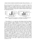
. As an example, consider the design of the gear
pair shown in Fig. 1.3, characterized by its face width b, number of teeth T
1
and
T
2
, center distance d, pressure angle ψ, tooth profile, and material. If center distance
d, pressure angle ψ, tooth profile, and material of the gears are fixed in advance,
these quantities can be called preassigned parameters. The remaining quantities can be
collectively represented by a design vector X = {x
1
, x
2
, x
3
}
T
= {b, T
1
, T
2
}

T
. If there are
no restrictions on the choice of b, T
1
, and T
2
, any set of three numbers will constitute a
design for the gear pair. If an n-dimensional Cartesian space with each coordinate axis
representing a design variable x
i
(i = 1, 2, . . . , n) is considered, the space is called
†
In the mathematical programming literature, the equality constraints l
j
(X) = 0, j = 1, 2, . . . , p are often
neglected, for simplicity, in the statement of a constrained optimization problem, although several methods
are available for handling problems with equality constraints.
1.4 Statement of an Optimization Problem 7
Figure 1.3 Gear pair in mesh.
the design variable space or simply design space. Each point in the n-dimensional
design space is called a design point and represents either a possible or an impossible
solution to the design problem. In the case of the design of a gear pair, the design
point {1.0, 20, 40}
T
, for example, represents a possible solution, whereas the design
point {1.0, −20, 40.5}
T
represents an impossible solution since it is not possible to
have either a negative value or a fractional value for the number of teeth.
1.4.2 Design Constraints

In many practical problems, the design variables cannot be chosen arbitrarily; rather,
they have to satisfy certain specified functional and other requirements. The restrictions
that must be satisfied to produce an acceptable design are collectively called design
constraints. Constraints that represent limitations on the behavior or performance of
the system are termed behavior or functional constraints. Constraints that represent
physical limitations on design variables, such as availability, fabricability, and trans-
portability, are known as geometric or side constraints. For example, for the gear pair
shown in Fig. 1.3, the face width b cannot be taken smaller than a certain value, due
to strength requirements. Similarly, the ratio of the numbers of teeth, T
1
/T
2
, is dictated
by the speeds of the input and output shafts, N
1
and N
2
. Since these constraints depend
on the performance of the gear pair, they are called behavior constraints. The values
of T
1
and T
2
cannot be any real numbers but can only be integers. Further, there can
be upper and lower bounds on T
1
and T
2
due to manufacturing limitations. Since these
constraints depend on the physical limitations, they are called side constraints.