Fisheries science JSFS tập 76, số 1, 2010 1

Fish Sci (2010) 76:1–11
DOI 10.1007/s12562-009-0186-x

ORIGINAL ARTICLE

Fisheries

Classification of fish schools based on evaluation
of acoustic descriptor characteristics
Aymen Charef • Seiji Ohshimo • Ichiro Aoki
Natheer Al Absi

•

Received: 27 May 2009 / Accepted: 15 October 2009 / Published online: 8 December 2009
Ó The Japanese Society of Fisheries Science 2009

Abstract Acoustic surveys were conducted from 2002 to
2006 in the East China Sea off the Japanese coast in order
to develop a quantitative classification typology of a
pelagic fish community and other co-occurring fishes based
on acoustic descriptors. Acoustic data were postprocessed
to detect and extract fish aggregations from echograms.
Based on the expert visual examination of the echograms,
detected schools were divided into three broad fish groups
according to their schooling characteristics and ethological
properties. Each fish school was described by a set of
associated descriptors in order to objectively allocate each
echo trace to its fish group. Two methods of supervised
classification were employed, the discriminant function

analysis (DFA) and the artificial neural network technique
(ANN). We evaluated and compared the performance of
both methods, which showed encouraging and about
equally highly correct classification rates (ANN 87.6%;
DFA 85.1%). In both techniques, positional and then
morphological parameters were most important in discriminating among fish schools. Fish catch composition
from midwater trawling validated the fish group classification through one representative example of each grouping. Both methods provided the essential information

A. Charef (&) Á I. Aoki
Graduate School of Agriculture and Life Science,
University of Tokyo, Bunkyo, Tokyo 113-8657, Japan
e-mail:
S. Ohshimo
Seikai National Fisheries Research Institute,
Fisheries Research Agency, Nagasaki 851-2213, Japan
N. Al Absi
Ocean Research Institute, University of Tokyo,
Nakano, Tokyo 164-8639, Japan

required for assessing fish stocks. Similar techniques of fish
classification might be applicable to marine ecosystems
with high pelagic fish diversity.
Keywords Acoustic descriptor Á Artificial neural
network Á Discriminant function analysis Á Fish
classification Á Species identification

Introduction
The northern part of the East China Sea represents one of
the main spawning and nursery areas of small pelagic
fishes in the waters off of the Japanese coast. It also constitutes an important fisheries ground for commercially

valuable pelagic fishes. During the last half decade, the
average landing was estimated to be roughly 250,000 tons
per year and was composed of Japanese anchovy Engraulis
japonicus, round herring Etrumeus teres, jack mackerel
Trachurus japonicus, chub mackerel Scomber japonicus
and spotted chub mackerel Scomber australasicus
(according to statistics from the Ministry of Agriculture,
Forestry and Fisheries, Government of Japan). The fish
stock size assessment is crucial for fisheries management in
these waters. Broadly, the main assessment techniques are
based on the virtual population analysis (VPA) method.
This method makes use of commercial catches, which
might bias the assessments and then generate very serious
overfishing problems [1, 2]. To eliminate such complications, reliable and fishery-independent data are needed.
Hydroacoustic methods are one of the few techniques
used in order to provide fisheries independent quantitative
estimates of fish stocks. Fisheries acoustics have experienced dramatic development in technologies and data
management. Acoustic surveys using quantitative scientific

123


2

echo sounders commonly employed to determine the
abundance and biomass of pelagic fish are becoming
increasingly important for the management of pelagic
fisheries [3]. Owing to the common aggregative behavior,
small pelagic species appear in echograms as a mixture of
diverse fish assemblages [4]. Echo integration is used to

estimate fish quantity since the sampled volume contains
overlapping target fish echoes [3]. The obtained target
strengths and the backscattering strength can be translated
into biomass units if the proportions of different species
and their length distribution and target strength on fish size
are known. In such a context, distinguishing among fish
targets is greatly needed to deal with each target fish echo
separately. Therefore, identification of echo traces of fish
schools is crucial in conjunction with accurate acoustic
surveys to give reliable estimates of target strength and
consequently improve the fish stock assessment.
The classification and subsequent identification of
acoustic targets to taxa or species are still the great challenge of fisheries acoustics [5, 6]. Species identification has
been limited by the difficulty in objectively classifying
backscattered energy of echo traces to species [6, 7]. Echotrace classification defined as the detection and description
of aggregations in acoustic data can be used to study
behavioral and ecological processes in aquatic environments [8]. It is generally agreed that besides integration of
target species’ biomass, useful information, such as features from digitized echograms, can be extracted from the
acoustic data. Many studies have attempted to develop
echo-trace classification in order to study shoaling behavior
and predator-prey interactions, to characterize fish aggregations, their spatial distribution and their relationship to
environmental variables; see Horne [9] for a review.
First attempts at fish identification introduced basically
subjective and time-consuming methods. These methods
involved expert scrutiny of echograms combined with
concurrent trawling data. Visual scrutiny of acoustic data
depends on human experience and is therefore subject to
biases and difficult to be quantified. This makes objective
methods more efficient, timely, less or not dependent on
subjective interpretation, and controlled by evaluating their

accuracy [10]. These automated methods require data
processing and detection of acoustic features from echograms as a first step, and secondly, description of selected
schools characteristics with a set of descriptors [11]. They
aim to train an algorithm on a set of identified, single
species schools. Then the algorithm is adopted to identify
other schools [12, 13]. Success of objective methods relies
primarily on a suitable choice of acoustic descriptors
concerning number and efficiency. In the case of high
diversity ecosystems, such as the East China Sea, where
small schools are numerous, species classification highly
depends on verification via trawl data.

123

Fish Sci (2010) 76:1–11

In the East China Sea, some attempts to estimate the
pelagic fish populations’ biomass were made with acoustic
surveys. These studies were restricted to subjective classification of fish species [14, 15], while limited to single
species such as anchovy [14, 16] and sardine [17, 18] in
other works. In this work, we applied two objective tools of
supervised echo-trace classification, discriminant function
analysis (DFA) and artificial neural network (ANN). The
aim of this paper is to describe and to evaluate the efficacy
of the two methods, based on a set of acoustic descriptors,
in objectively classifying fish schools of pelagic fish
community and other co-occurring fishes such as pearlside
and lantern fish.

Materials and methods

Data collection
Acoustic surveys were conducted annually in the late
summer from 2002 to 2006 by the Japanese Fisheries
Research Agency on board the RV Yoko Maru. Surveys
were carried out along 27 parallel transects spaced by 10
nautical miles (Fig. 1). During surveys, vessel speed was
approximately 10 knots and total length of transects ranged
from 593 to 828 nautical miles (Table 1).

Fig. 1 Study area and acoustic survey scheme


Fish Sci (2010) 76:1–11
Table 1 Year, beginning and
end dates, total length of
transects, number of detected
schools and number of stations
of CTD casts and midwater
trawls during each acoustic
survey

3

Year

Begin date

End date

Total length of transects

(nautical miles)

Number of
detected schools

Number
of stations

2002

22 August

24 September

828

221

17

2003

27 August

25 September

828

187

21

2004

24 August

12 September

593

163

12

2005

24 August

10 September

805

168

18

2006

23 August

7 September

791

91

20

Acoustic data were collected using a calibrated hullmounted SIMRAD EK505 scientific echo-sounder system
operating at 38 kHz with a time-varied gain function set
at 20 log R. The echo-sounder pulse length was 1 ms, its
ping rate was 0.33 ping s-1, and its estimated sound
speed 1500 ms-1, giving a target resolution of 0.001 s 9
1500 m s-1/2 = 0.75 m. Acoustic measurements were
logged continuously during all surveys and recorded only
during daytime.
Small pelagic fish species may reduce the risk of daytime
predation by schooling [19]. The schooling behavior typically characterizes each fish school in daylight, which is
essential for the fish identification. However, during twilight
and nighttime, fish schools scatter and overlap, which biases
the fish identification in acoustic processing [4, 20].
Acoustic data processing
Acoustic data were postprocessed using Echoview Software version 4.50 [21]. The seafloor was automatically
detected using the ‘‘maximum Sv backstep’’ algorithm,
where the backstep was set at 1 m. Data deeper than 1 m
above the selected bottom line were removed due to the
false bottom detection. Data shallower than 10 m were also
removed from analyses to eliminate the transmit pulse and
reduce backscatter by surface bubbles.
A background threshold of -67 dB was applied equivalently to all echograms. The threshold was determined by

analyzing a subset of data collected from each year and
allowed accurate detection of all possible aggregations of
target fishes. Fish aggregations were detected and characterized using the ‘‘Schools detection’’ module implemented
in Echoview. Input parameters were set according to
schools’ features observed in acoustic records. The algorithm pattern required schools to be at least 8 m long and
4 m high. Adjacent aggregations were linked to shape one
school if the maximum horizontal linking distance was
15 m and maximum vertical connection distance 5 m.
Then echograms were visually inspected, and doubtful and
‘false’ detections (scattering layer, acoustic interference)
were removed. Connected aggregations with dimensions
smaller than the minimum school length and height
parameters were discarded.

For each detected acoustic target, a set of five school
descriptors was calculated and extracted, and they fell into
three categories (Table 2): (1) morphological: school
length, height and height mean; (2) energetic: mean volume backscattering strength (Sv); (3) positional: mean
school altitude (Depth).
Midwater trawl catch data
Midwater trawling was used to identify acoustic targets and
to establish their weight composition. Midwater trawling
was only performed at nighttime because of the high netavoidance rate of fish targets in the daytime, which makes
it difficult to sample the observed fish schools in acoustic
recordings [22]. Visual inspection of echograms for several
hours permitted the characterization of schooling behavior
and swimming depth of target species. The position of the

Table 2 Definitions and units of school descriptors used in both
analysis methods

Descriptor

Unit

Indication

Length

m

Height

m

The horizontal distance
along the transect from
the first to last ping
crossing the school
The vertical distance
separating the maximum
and minimum depths of
the rectangle bounding
the school

Height mean

m

The mean distance from the
upper to lower limit along

each ping crossing the fish
school

dB

The mean energy produced
by pixels shaping a fish
school, which indicates its
mean density

m

The distance from the sea
surface to the geometric
center of the fish school

Morphological

Energetic
Mean volume
backscattering
strength (Sv)
Positional
Mean school
depth (Depth)

123


4

Fish Sci (2010) 76:1–11

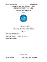
Fig. 2 Acoustic recordings showing typical schools of three different fish groups

trawl stations was decided beforehand according to the
location of peculiar fish concentrations detected during
acoustic surveys in the daytime.
A total of 88 midwater trawls were conducted (Table 1).
Towing speed was approximately 3 knots for a towing time
of 30 min. Towing depth was targeted to fish schools by
adjusting the towing speed and warp length. The mouth of
the trawl net was approximately 20 m by 20 m, and the
mesh sizes of the cod end and the inner bag were 60 and
20 mm, respectively. The trawl catch was separated by
species, and the total weight of each species was
determined.
Other data
Conductivity-temperature-depth (CTD) profiles were taken
along the survey tracks at the beginning of each trawling
operation. The on-board data recording and entry system
was deployed to record series of time (GMT), geographic
position and the EK 500 vessel log.
Fish-group classification
School images were selected and allocated to a species
through visual expert examination of the echogram displays based on prior experience knowledge, in conjunction
with the interpretation of echograms. The identified target
fishes were classified into three types of fish groups
according to their schooling characteristics and ethological
properties. The verification of this typology also involved

the results of the midwater trawl catch amount and
composition.
The classification was partially based on the previous
findings of Ohshimo [15] from acoustics surveys conducted
following a similar survey scheme on the same study area.
The first type (G1) consisted of compactly aggregated
schools, assumed to be Japanese anchovy and round herring, within the upper layer of the water column. The

123

second group (G2) appeared in the midwater layers, mostly
above the bottom rise structure, and it was thought to be
composed of jack mackerel and chub mackerel. The last
group (G3), assumed to consist of lantern fish and pearlside, occurred in demersal layers mainly along slopes and
formed horizontally elongated schools in contact with the
seabed (Fig. 2). Some detected fish schools that did not fall
within this typology were neglected.
Statistical analysis
Discriminant function analysis (DFA) is a well-known
statistical procedure used to predict group membership
based on a combination of the interval variable [23]. The
five school descriptors constituted the predictor variables
for this discrimination analysis, whereas the dependent
variable was fish group (G1, G2, G3) defined a priori on the
basis of visual expert scrutiny and direct sampling results.
DFA was performed using SPSS (version 6.0) based on
Mahalanobis distances (D). Mahalanobis distance is the
distance between a case and the centroid for each fish
group (of the dependent variable) in attribute space. By this
procedure, each school is allocated to the fish group for

which D has the smallest value [24]. Classification accuracy was estimated with leave-one-out cross-validation, in
which the discriminant function is first derived from only
n - 1 schools and then used to classify the other school
left out. The procedure is repeated n times, each time
omitting a different observation [25]. DFA was applied for
overall years data pooled together.
Artificial neural networks
Artificial neural networks (ANN) were also used as the
method of species classification and identification of fish
schools from acoustic data. They imitate human neuron
functioning and solve problems by applying knowledge
gained from past experience to new situations [26].


Fish Sci (2010) 76:1–11

5

Results
Classification using discriminant function analysis

Fig. 3 Network architecture for the model used in this study

A multiple layer perceptrons (MLPs) neural network
was constructed and computed using Matlab 6.0. MLPs are
the most commonly and the simplest network type used,
primarily due to their speed and versatility [27]. They
consist of three feed-forward layers: input, hidden and
output (Fig. 3). The input layer was composed of five
variables. The number of nodes in the hidden layer was

determined by testing the performance of the model using a
range of node numbers. The dependent variable fish groups
represented the output layer. The data set was split into a
training set and validation set consisting of 70 and 30% of
the identified schools, respectively, with the same proportion of each fish group. Based on supervised learning, the
neural network was trained by means of a backpropagation
learning algorithm (BP) in order to develop the ability to
correctly classify new fish schools from further acoustic
data [28]. The school fish’s classifications based on their
relative descriptors occurred in two major phases. First,
during the learning phase, internal parameters within the
network were adjusted iteratively. The performance of the
network, equivalent to classifying schools into fish groups
accurately, was maximized; this stage continued until there
was no further increase in network performance or classification success. Although the aim of the training is to
reduce the error as much as possible, reducing the error too
much leads to the network learning the noise rather than
underlying relationships. Precautions were taken to avoid
over-fitting (over-training) of the network’s model. Finally,
during the validation phase, which is the second phase, the
optimal network was applied to test sets, along with crossvalidation.

Discriminant function analysis was computed using 830
detected schools and five acoustic descriptors (Tables 1, 3).
Since the dependent variable, fish school, has three groups,
two canonical discriminant functions were determined.
Both functions were significant, but nearly all of the variance in the model is captured by the first discriminant
function. The small Wilk’s lambda coefficients indicated
also that only the first function is useful. The eigenvalues
confirmed the significant difference between both discriminant functions. The standardized discriminant function coefficients were used to compare descriptors

measured on different scales. Coefficients with large
absolute value correspond to variables with greater discriminating ability. This implies that within the first function, for instance, depth contributed the most. Thus,
descriptors in rank order of efficacy in discriminating fish
schools are depth, height, height mean and length, while
mean volume backscattering strength Sv comes last.
The confusion matrix showed the results of the DFA
using five acoustic descriptors for discriminating fish
schools from survey data of 5 years (Table 4). Emboldened
values on the main diagonal of each confusion matrix
represent the number of schools that were correctly identified within every fish group. The overall correct classification was evaluated at 85.1%.
The correct recognition rates per group showed high
scores for G1 schools. Almost 95% were well assigned and
distinguished from other groups. G2 schools represent 57%
of the total number of schools and were the least correctly
classified with a relatively low rate of 80.3%. The proportion of G3 schools is small, with only 13.25%, and had a
correct classification score of 81.8%.
Classification using an artificial neural network
Application of the trained network to 5 years of pooled
acoustic data resulted in predicted species compositions
that corresponded well to those observed with an overall
correct classification evaluated at 87.6% for the validation
data set (Table 5). The model performed well for

Table 3 Results of discriminant analysis using five descriptors for overall 5 years data
Analyzed school
group discriminant
function

Wilk’s k

First function
Second function

% of
variance

Eigenvalue

0.269

94.6

2.291

0.885

5.4

0.130

Standardized canonical discriminant function coefficient
Depth

Sv

Significance
level

Height

Height mean

Length

0.971

0.305

-0.304

0.158

0.043

0.000

-0.296

0.537

-0.424

0.835

-0.093

0.000

123

6

Fish Sci (2010) 76:1–11

Table 4 Confusion matrix of DFA analysis
Predicted group
G1

G2

Total

% Correct

G3

Observed group
G1

234

10

0

244

95.9

G2

62

382

32

476

80.3

G3
Overall

5

15

90

110

81.8

301

407

122

830

85.1

Number of schools from each group (true classification) distributed
over predicted groups. Values in bold denote correctly classified
schools

Fig. 4 Proportion of the contribution factor of each descriptor used
as input into the artificial neural network

Table 5 Results of ANN classification from the two data sets
Predicted group
G1

G2

Total

% Correct

97.7

G3

Observed group
Training data set
G1

169

3

1

173

G2

21

297

13

331

89.7

G3

1

6

69

76

90.8

Overall
191
Validation data set

306

83

580

92.2

G1

71

3

0

74

95.9

G2

15

120

8

143

83.9

G3

1

4

28

33

84.8

87

127

36

250

87.6

Overall

Values in bold represent correct assignment

classifying G1 schools with a correct classification rate of
95.94%, but less for G3 and G2 schools, with 84.84 and
83.91%, respectively.
The contribution factor of a variable is the sum of the
absolute values of the weights generated from this particular variable. It reveals the importance of input variables,
descriptors, to classify fish schools. The analysis showed
similar ordering of descriptor categories to DFA results and
indicated that the heaviest impact in classifying was
assigned to positional, morphological and then energetic
properties of a school. However, the ascending order within
the morphological descriptors category differs slightly,
though depth was the most efficient descriptor (Fig. 4).
Validation with catch data
Midwater trawling catch assisted in fish identification
simultaneously with visual scrutiny of echograms. The
recorded acoustic data in daytime permitted to observe
typical shapes of fish schools and then facilitated their

123

identification. Examination of catch data over all 88 tows
showed that the dominant target species was jack mackerel,
which contributed 22% by weight of the total catch, followed by Japanese anchovy (18.4%) and lantern fishes
(16%) (Table 6). Round herring was an exception in 2002
and was the most abundant species, reaching 20% of the
total catch by weight in the same year. The non-target

species that did not fall in the three identified categories of
major species were clustered into one group as ‘‘others’’
and represented around 28% of the total catch amount
(Table 6). Catch composition was also valuable to verify
the classification of target species into three groups of fish
schools. Table 7 shows catch composition data from
selected trawls hauled near the locations where schools of
G1, G2 or G3 were observed in daytime. Each group of
species was assigned according to the most dominant
species comprised in each trawl catch.
A summary of trawl hauls with fish schools matching
with acoustically detected schools is shown in Table 8.
Looking at both tables simultaneously (Tables 7, 8) permitted examining the catch composition according to the
amount and number of trawl hauls. In the overall data for
5 years, the number of detected schools evenly matched
with the catch amount of target species. The correspondence between detected and caught G1 schools was estimated to be 44% of the catch from 11 hauls, mainly made
up of Japanese anchovy as it is the most abundant species
in G1. The mismatch is primarily due to the high amount of
catch of the G2 and G3 species. Around 34% of the
detected G2 schools were validated by catch data from 11
hauls. Other co-occurring species, mainly represented by
puffer fishes and squid, made up 43% of the total catch
amount and were fairly abundant in 15 hauls; some of them
were small catches (less than 2 kg). In the case of G3
schools, nearly 41% of identified schools were validated by
catch results. Bycatch species that were caught during the
same trawl hauls represented 33% of the total catch but
belonged to one trawl haul.

Fish Sci (2010) 76:1–11

7

Table 6 Catch amount (kg) by midwater trawling of abundant species assumed to compose acoustically detected fish schools
Fish group

Species

2002

2003

2004

Engraulis japonicus Japanese anchovy

44.2 (13.4)

7.2 (1.8)

55.4 (42.0) 36.9 (9.3)

Etrumeus teres

Round herring

67.7 (20.5)

10.8 (2.7)

0.9 (0.7)

5.5 (1.4)

23.0 (1.8)

107.8 (7.0)

Sardinops
melanostictus
Decapterus
macrosoma

Japanese sardine

0

0.1 (0.03)

0.1 (0.1)

0.1 (0.03)

0.7 (0.2)

1.0 (0.1)

Shortfin scad

7.3 (2.2)

6.4 (1.6)

3.4 (2.6)

0.9 (0.2)

3.0 (1.1)

21.0 (1.4)

Decapterus
maruadsi

Round scad

0

0.2 (0.1)

0

28.1 (7.1)

0.3 (0.1)

28.6 (1.9)

Scomber japonicus

Chub mackerel

2.1 (0.6)

0.5 (0.1)

0.6 (0.5)

8.4 (2.1)

0

11.6 (0.8)

Scomber
austratasicus

Spotted chub
mackerel

0

0

2.8 (2.1)

8.4 (2.1)

5.6 (2.0)

16.8 (1.1)

Trachurus
japonicus

Japanese jack
mackerel

38.6 (11.7)

215.1 (54.2) 35.0 (26.5) 37.6 (9.5)

15.1 (5.3)

341.4 (22.2)

Diaphus spp

Lantern fishes

0

43.3 (10.9)

3.8 (2.9)

191.7 (48.5) 7.3 (2.6)

246.1 (16.0)

Maurolicus
japonicus

Pearlside

0.8 (0.2)

0.1 (0.03)

0.1 (0.1)

50.2 (12.7)

51.3 (3.3)

Arothron spp

Puffer fishes

113.8 (34.4) 60.6 (15.3)

8.6 (6.5)

0.8 (0.2)

0.6 (0.2)

184.3 (12.0)

Auxis rochei

Bullet tuna

6.3 (1.9)

0

0

1.9 (0.5)

3.9 (1.4)

12.1 (0.8)

Diodon hystrix
Loglio edulis

Porcupinefish
Swordtip squid

0.9 (0.3)
5.9 (1.8)

0.2 (0.1)
8.7 (2.2)

0
8.3 (6.3)

0
16.6 (4.2)

32.0 (11.2)
14.4 (5.1)

33.1 (2.2)
53.8 (3.5)

Psenopsis anomala

Melon seed

Scientific name
G1

G2

G3

Others

2005

2006

Total

Common name

139.7 (49.1) 283.4 (18.4)

0.1 (0.4)

0.2 (0.1)

1.7 (0.4)

0

5.9 (1.5)

4.7 (1.7)

12.4 (0.8)

Todarodes pacificus Japanese common
squid

6.7 (2.0)

2.6 (0.7)

0.7 (0.5)

2.0 (0.5)

1.6 (0.6)

13.5 (0.9)

Others

36.4 (11.0)

39.3 (9.9)

12.4 (9.4)

0.8 (0.2)

32.7 (11.5)

121.5 (7.9)

330.9

396.8

131.9

395.4

284.5

1539.5

Total catch
of all
species

Values between brackets represent percentage (%)

Table 7 Comparison of acoustically detected schools with trawl catch composition
Fish Number Caught species
group of hauls
G1
Japanese
Anchovy

G2
Round
Herring

Japanese
sardine

G3

Scomber
spp.

Trachurus
spp.

Decapterus
spp.

1.2 (0.3%)

142.2 (31.3%) 2 (0.4%)

Lantern
fishes

Pearlside

Others

Detected schools
G1

11

184.6 (40.7%) 16.5 (3.6%) 0.5 (0.1%)

G2

28

58.6 (11.9%)

28.3 (7.3%) 0.05 (0.01%) 11.7 (2.4%) 138.7 (28.1%) 20.2 (4.1%) 22.8 (4.6%)

G3

7

10.4 (5%)

41 (19.7%)

0

0.2 (0.1%)

0

2.1 (1%)

92.4 (20.4%) 0.1 (0.02%) 30.35 (6.7%)
0.1 (0.02%) 213.42 (43.2%)

34.2 (16.4%) 51 (24.5%) 69.45 (33.3%)

Upper line of each row represents catch amount per kg. Lower line indicates percentage of catch amount
Values in bold represent fish species included in each group

Discussion
Comparison of classification techniques
In this study, ANN and DFA models were optimized in
order to classify fish schools. Both techniques showed
nearly similar recognition performance. The overall classification rate was higher for ANN than DFA, but

nevertheless was only slightly higher. As for the three fish
groups’ relative classifications, there were minor differences in classification success based on the two specified
methods. In particular, differences were trivial for G1
schools, whereas the successes of discrimination of G2 and
G3 schools were significantly more important with ANN
than DFA (Tables 4, 5). The particularly effective power of
ANN to classify fish schools is attributed to its ability to

123


8

Fish Sci (2010) 76:1–11

Table 8 Summary of acoustically detected schools with the most
abundant caught species in number of trawl hauls
Caught species
G1

G2

Total
G3

Others

Detected schools

a

G1

6

1

2

2

11

G2
G3

4
3

11
0

1
3

15a
1

28
7

Five hauls scored less than 2 kg of total catch per haul

handle non-linear relationships between descriptors and
dependent variables, through the presence of many intervening information-processing units, which each uses the
binary logistic activation function [27]. A further advantage of ANN is the small impact of extreme values on
discrimination success and the absence of any specific

assumptions on the distribution of the data. In fact, ANN
established functional relationships of the data by learning
from the input training data set [29, 30]. On the other hand,
despite these advantages, a liability of its application is that
it needed much more computing time than discriminant
analysis, especially during optimization procedures such as
weight analysis.
Similar performances of ANN and DFA in identifying
fish schools that have been found in several studies corroborate our finding that ANN is more effective than DFA
[12, 13, 31]. Moreover, they reported better, sometimes far
better, overall classification rates. These mentioned case
studies inferred that an increasing number of descriptors
should lead to an improvement in discrimination effectiveness. However, Scalabrin et al. [32] found a lower rate
when classifying only three species using nine school
parameters. Theoretically, the greater the number of
parameters that can be included in the model, the more
likely the analysis will assign a school image to the correct
group [13]. However, in our practical analysis, for both
classification methods we were limited to five acoustic
descriptors as input variables.
Parameters controlling fish-group classification
The fish schools’ classification is defined as the discrimination of acoustic backscatters to the species, genus or
group level, depending on the richness of fish diversity
[10]. In this work, the classification of fish echo traces into
three fish groups was reliable due to the high fish diversity
in the East China Sea. The acoustic aggregations of the
numerous target species were categorized based solely on
their schooling characteristics. The feasibility of this
approach is justified by the existence of acoustic populations; groups of echo traces show a consistent pattern in

123

space and time at a regional scale [33]. In tropical waters,
Gerlotto succeeded in dividing highly multispecific fish
communities into four fish acoustic populations [34].
However, for some marine systems at high latitudes, such
as the North Atlantic Ocean, species richness is relatively
poor. The low number of target fishes and the occurrence of
monospecific schools permitted a lower level of discrimination and yielded a higher successful classification rate
[32].
The vertical distribution of fish schools in the water
column gave evidence of the typology applied in this
study. G1 schools existed predominantly in the upper
layer of the water column above the thermocline detected
at approximately 50 m depth (Fig. 5a). The G2 schools
were observed within a deeper layer below the thermocline. G3 schools were distributed in the bottom half of the
water column below 150 m depth until the closest layer to
the sea bottom. The vertical distribution of G3 species is
in agreement with the vertical range (160–200 m) reported by Fujino et al. [35] in the case of pearlsides and below
200 m depth in the case of mesopelagic lantern fishes
[36].
The vertical distribution of fish schools exhibited a
noticeable pattern that corresponds to the overlap of G1–
G2 schools and G2–G3 schools in water layers at 60–80
and 160–180 m, respectively. Fish schools co-occurring
within these depths could not be discriminated properly on
the basis of the positional descriptor. Both methods (DFA
and ANN) resulted in relatively weaker performance
within these overlap layers; the correct classification rate
did not exceed 88%.

Notwithstanding the fair limitation of fish-group classification within ‘overlap’ layers, the results of DFA and
ANN revealed that the school’s altitude in the water column was the most effective acoustic descriptor in successfully discriminating schools into the three groups. On
the other hand, morphological acoustic descriptors and
backscattered volume Sv contributed to distinguishing
among species. In fact, the G3 species pearlsides and lantern fishes formed generally large elongated aggregations
that were fairly dense and characterized by relatively low
Sv values. The G2 species jack mackerel, spotted mackerel
and chub mackerel aggregated in relatively smaller schools
marked by higher Sv values (Fig. 5b, c, d).
Although the vertical distribution of the target fishes
cannot be addressed in detail within the scope of this paper,
it provided valuable information about the environmental
and physiological properties of identified target species.
The occurrence of Japanese anchovy, Japanese sardine and
round herring above the thermocline was most likely
related to temperature gradient patterns. Temperature at the
sea surface varied between surveys from 26.5 to 28.8°C
(Fig. 6), and below 60 m depth, temperature profiles were


Fish Sci (2010) 76:1–11

9

facilitated the identification of species confined to the
upper layers [14].
The availability of food as well as avoidance of predation could also be plausible key factors concerning the
vertical distribution patterns [37]. Small fish may have
migrated to a depth level with a lower concentration of
larger fish to avoid predation [36]. Myctophids and pearlsides fishes feed on zooplankton. They ascend from the sea

bottom at night following food and prey patterns and are
thought to compete for food with pelagic fish within the
upper layer [14, 15].
Fish identification improvement

Fig. 5 Distribution of detected schools in relation to depth (a),
height (b), length (c) and mean backscatter volume Sv (d)

fairly homogenous. The thermocline might have played the
role of a barrier that restricted the migration of these species to deeper layers. Thus, the thermal barrier implicitly

Several works have been using multiple frequency echo
sounding to allocate fish echoes to species by using the
frequency difference in mean volume backscattering
strength (MVBS) and target strength differencing [38–40].
These methods have shown considerable promise and
provided high rates of correct classification in restricted
ecological situations, that is, none have provided a classifier that can be applied over broad ranges of time and space
[41]. In the East China Sea particularly, owing to the high
fish diversity, the use of an extended number of narrowband acoustic frequencies may facilitate the identification
of fish species. More precisely, low frequencies might be
the best aid to increase species discrimination, for instance,
midwater layers of mesopelagic fish appear much stronger
on 12 kHz than on 38 kHz [42–44]. Simultaneously, with
more accurate acoustic surveys, additional trawl data
should facilitate the identification of fish species within
each group. In parallel, the increase in the amount of collected data enhances ANN training and thus its efficacy.
Taking the advantage of its fast performance and the speed
of processing using modern computers, the application of
ANNs in real-time classification would be advantageous in

fisheries stock assessments.
In the same order of magnitude, further statistical
analysis should be performed to evaluate the consistency of
acoustic data and trawl data. Ideally, the fish schools
detected during daylight acoustic surveys will be caught
using the midwater trawling conducted only at nighttime.
The horizontal migration of fish may bias the verification
of identified fish schools using trawl data. However, in this
work, the time lag was neglected since midwater stations
were meticulously chosen to correspond to locations of
target fish schools observed previously in echograms.
Quantification of uncertainty of the match between both
data sets (acoustic and trawl data) may lead to improving
the objectivity of fish identification and classification.
In conclusion, this study demonstrated that the neural
network can perform reasonably well in classifying fish
schools and that it performs slightly better than DFA. This

123


10

Fish Sci (2010) 76:1–11

substitute for rather than a necessary complement to conventional survey methods.
Acknowledgments We are grateful to Dr. Hiroshige Tanaka
(Fisheries Research Agency) for data collection, and Dr. Tadanori
Fujino and Dr. Kazushi Miyashita (University of Hokkaido) for data
analysis initiation. Thanks are due to Dr. Vidar Wespestad (University

of Alaska Fairbanks), Dr. Hideaki Tanoue and Dr. Teruhisa Komatsu
(University of Tokyo) for providing advice at various stages of the
work. We thank Dr. Takaomi Kaneko for his thorough editorial
assistance.

References

Fig. 6 Vertical profiles of temperature during surveys

achievement was guaranteed by an integration of prior
knowledge, direct sampling in conjunction with the two
patterns of recognition and classification. More specifically, the use of a set of five descriptors that combines
positional, energetic and morphologic criteria provided the
best fish-group discrimination. The choice was made to
cover many aspects of the school while avoiding parameters likely to generate redundant information. In our practical analysis, for both methods, we concluded that
compiling a different set of descriptors and adding other
acoustic parameters (such as skewness and school elongation) during model optimization led to a decrease in the
overall classification rate. In some studies, more complex
criteria were implemented to parameterize the shape and
intrinsic structure complexity of the school [13, 41]. These
authors recognized that using such descriptors is satisfactory for classification purposes for large schools, but likely
to become not valuable to some extent for smaller schools.
This study succeeded in potentially improving the
objectivity of the identification and discrimination of fish
species, illustrated by high correct classification rates
accounting for both tools of analysis. Further work on these
approaches should continue with an expanded acoustic data
set for all species of the three groups. Subsequently, these
two methods will represent powerful means able to
increase the accuracy of the stock size assessment in the

East China Sea using hydroacoustic techniques. For the
foreseeable future, acoustic surveys must be viewed as a

123

1. Hansson S (1999) Human effects on the Baltic Sea ecosystem—
fishing and eutrophication. In: Anonymous (eds) Ecosystem
approaches for fisheries management. Fairbanks University of
Alaska, pp 405–406
2. Kuikka S, Hilden M, Gislason H, Hansson S, Sparholt H, Varis O
(1999) Modelling environmentally driven uncertainties in Baltic
Cod management by Bayesian influence diagrams. Can J Fish
Aquat Sci 56:629–641
3. Simmonds J, MacLennan D (2005) Fisheries acoustics: theory
and practice, 2nd edn. Blackwell, Oxford
4. Brehmer P, Gerlotto F, Laurent C, Cotel P, Achury A, Samb B
(2007) Schooling behaviour of small pelagic fish: phenotypic
expression of independent stimuli. Mar Ecol Prog Ser 334:263–272
5. MacLennan DN, Holliday DV (1996) Fisheries and plankton
acoustics: past, present, and future. ICES J Mar Sci 53:513–516
6. Mackinson S, Freeman S, Flatt R, Meadows B (2004) Improved
acoustic surveys that save time and money: integrating fisheries
and ground-discrimination acoustic technologies. J Exp Mar Biol
Ecol 305:129–140
7. Lundgren B, Nielsen JR (2008) A method for the possible species
discrimination of juvenile gadoids by broad-bandwidth
backscattering spectra vs. angle of incidence. ICES J Mar Sci
65:581–593
8. ICES (2000) Report on echo trace classification. ICES Cooperative Research Report, Denmark
9. Horne J (2000) Acoustic approaches to remote species identification: a review. Fish Oceanogr 9:356–371

10. Jech JM, Michaels WL (2006) A multifrequency method to
classify and evaluate fisheries acoustics data. Can J Fish Aquat
Sci 63:2225–2235
11. Reid D, Scalabrin C, Petitgas P, Masse J, Aukland R, Carrera P,
Georgakarakos S (2000) Standard protocols for the analysis
of school based data from echo sounder surveys. Fish Res 47:
125–136
12. Simmonds EJ, Armstrong F, Copland PJ (1996) Species identification using wideband backscatter with neural network and
discriminant analysis. ICES J Mar Sci 53:189–195
13. Haralabous J, Georgakarakos S (1996) Artificial neural networks
as a tool for species identification of fish schools. ICES J Mar Sci
53:173–180
14. Ohshimo S (1996) Acoustic estimation of biomass and school
character of anchovy Engraulis japonicus in the East China Sea
and the Yellow Sea. Fish Sci 62:344–349
15. Ohshimo S (2004) Spatial distribution and biomass of pelagic fish
in the East China Sea in summer, based on acoustic surveys from
1997 to 2001. Fish Sci 70:389–400
16. Iversen SA, Zhu D, Johannessen A, Toresen R (1993) Stock size,
distribution and biology of anchovy in the Yellow Sea and East
China Sea. Fish Res 16:147–163


Fish Sci (2010) 76:1–11
17. Takeshita K, Ogawa N, Mitani T, Hamada R, Inui E, Kubota K
(1988) Acoustic surveys of spawning sardine, Sardinops melanosticta, in the coastal waters of west Japan. Bull Seikai Reg
Fish Res Lab 66:101–117
18. Ohshimo S, Mitani T, Honda S (1998) Acoustic surveys of
spawning sardine Sardinops melanostictus in the waters off
western and southern Kyushu, Japan. Fish Sci 64:665–672

19. Connell SD (2000) Is there safety in numbers for prey? Oikos
88:527–532
20. Sassa C, Moser HG, Kawaguchi K (2002) Horizontal and vertical
distribution patterns of larval myctophid fishes in the Kuroshio
Current region. Fish Oceanogr 11:1–10
21. Myriax (2007) Echoview. Version 4.50. Myriax software Pty Ltd
1995–2008
22. Suuronen P, Lehtonen E, Wallace J (1997) Avoidance and escape
behaviour by herring encountering midwater trawls. Fish Res
29:13–24
23. Duda RO, Hart PE, Stork DG (2001) Pattern classification, 2nd
edn. Wiley, London
24. McLachlan GJ (2004) Discriminant analysis and statistical pattern recognition. Wiley, NY
25. Landau S, Everitt BS (2004) A handbook of statistical analyses
using SPSS. Chapman & Hall/CRC, London
26. Arbib M (2003) The handbook of brain theory and neural networks, 2nd edn. MIT Press, Cambridge
27. Basheer IA, Hajmeer M (2000) Artificial neural networks: fundamentals, computing, design, and application. J Microbiol
Methods 43:3–31
28. Rumelhart DE, Hinton GE, Williams RJ (1986) Learning representations by back-propagating errors. Nature 323:533–536
29. Chen DG, Ware DM (1999) A neural network model for forecasting
fish stock recruitment. Can J Fish Aquat Sci 56:2385–2396
30. Cabreira AG, Tripode M, Madirolas A (2009) Artificial neural networks for fish-species identification. ICES J Mar Sci 66:1119–1129
31. Woodd-Walker RS, Watkins JL, Brierley AS (2003) Identification of Southern Ocean acoustic targets using aggregation backscatter and shape characteristics. ICES J Mar Sci 60:641–649
32. Scalabrin C, Diner N, Weill A, Hillion A, Mouchot MC (1996)
Narrowband acoustic identification of monospecific fish shoals.
ICES J Mar Sci 53:181–188

11
33. Petitgas P, Masse J, Beillois P, Lebarbier E, Le Cann A (2003)
Sampling variance of species identification in fisheries-acoustic

surveys based on automated procedures associating acoustic
images and trawl hauls. ICES J Mar Sci 60:437–445
34. Gerlotto F (1993) Identification and spatial stratification of
tropical fish concentrations using acoustic populations. Aquat
Living Resour 6:243–254
35. Fujino T, Miyashita K, Aoki I, Masuda S, Uji R, Shimura T
(2005) Acoustic identification of scattering layer by Maurolicus
japonicus around the Oki Islands, Sea of Japan. Nippon Suisan
Gakkaishi 71:947–956 (in Japanese with English abstract)
36. Watanabe H, Moku M, Kawaguchi K, Ishimaru K, Ohno A
(1999) Diel vertical migration of myctophid fishes (Family Myctophidae) in the transitional waters of the western North Pacific.
Fish Oceanogr 8:115–127
37. Zwolinski J, Morais A, Marques V, Stratoudakis Y, Fernandes
PG (2007) Diel variation in the vertical distribution and schooling
behaviour of sardine (Sardina pilchardus) off Portugal. ICES J
Mar Sci 64:963–972
38. Anderson CIH, Horne JK, Boyle J (2007) Applying a robust
probabilistic classification technique to multi-frequency fisheries
acoustics data. J Acoust Soc Am 121:EL230–EL237
39. Kang M, Furusawa M, Miyashita K (2002) Effective and accurate
use of difference in mean volume backscattering strength to
identify fish and plankton. ICES J Mar Sci 59:794–804
40. Gauthier S, Horne JK (2004) Potential acoustic discrimination
within boreal fish assemblages. ICES J Mar Sci 61:836–845
41. LeFeuvre P, Rose GA, Gosine R, Hale R, Pearson W, Khan R
(2000) Acoustic species identification in the Northwest Atlantic
using digital image processing. Fish Res 47:137–147
42. Barr R (2000) A design study of an acoustic system for differentiating orange roughy and other New Zealand deepwater species. J Acoust Soc Am 109:164–178
43. O’Driscoll RL (2003) Determining species composition in
mixed-species marks: an example from the New Zealand hoki

(Macruronus novaezelandiae) fishery. ICES J Mar Sci 60:609–
616
44. Nero RW, Magnuson JJ (1989) Characterization of patches along
transects using high resolution 70-kHz integrated echo data. Can
J Fish Aquat Sci 46:2056–2064

123


Fish Sci (2010) 76:13–20
DOI 10.1007/s12562-009-0194-x

ORIGINAL ARTICLE

Fisheries

Acoustic pressure sensitivities and effects of particle
motion in red sea bream Pagrus major
Takahito Kojima • Tomohiro Suga • Akitsu Kusano •
Saeko Shimizu • Haruna Matsumoto • Shinichi Aoki •
Noriyuki Takai • Toru Taniuchi

Received: 30 April 2009 / Accepted: 2 November 2009 / Published online: 15 December 2009
Ó The Japanese Society of Fisheries Science 2009

Abstract The auditory pressure thresholds of red sea
bream were examined using cardiac response in the field by
placing fish subjects far from the sound source to prevent
particle motion. Pressure and particle motion thresholds
were also obtained using the auditory brainstem response

(ABR) technique. The thresholds at 100 and 200 Hz were
significantly higher when measured using the cardiac
response in the far field than those obtained in previously
conducted experiments in experimental tub. However,
thresholds obtained using ABR from 200 to 500 Hz were
not remarkably lower, although significantly different
(0.01 \ P \ 0.05), compared with those obtained using
cardiac response in the far field. Furthermore, calculated
particle velocity thresholds indicated that fish probably
detected particle motion within the frequency range of
50–200 Hz, even in fish with a deactivated lateral line.
Although the ABR method is widely applied in fish auditory study, hearing thresholds are apparently affected by
particle motion.
Keywords ABR Á Audiogram Á Dipole Á Far field Á
Inner ear Á Lateral line Á Near field
T. Kojima (&) Á A. Kusano Á S. Shimizu Á H. Matsumoto Á
S. Aoki Á N. Takai Á T. Taniuchi
College of Bioresource Sciences, Nihon University,
Fujisawa, Kanagawa 252-8510, Japan
e-mail:
T. Suga
Graduate School of Fisheries Science, Hokkaido University,
Hakodate, Hokkaido 041-8611, Japan
Present Address:
T. Suga
National Research Institute of Fisheries Engineering,
Kamisu, Ibaraki 314-0408, Japan

Introduction
Auditory stimuli to control the behavior, activity, and physiological condition of fish in coastal waters or culturing

facilities have persistently been targeted for investigation [1].
Fish have been conditioned to be attracted by sound upon
emission of a signal for marine ranching [2, 3]. When a sound
signal is emitted in water, water particle motion attenuates
faster than pressure waves because pressure decreases linearly while displacement decreases with the square of the
distance from the source according to the acoustic law [4, 5].
Consequently, in the field, it is difficult to propagate particle
motion to fish from a distant sound source. Therefore, it might
be more important to evaluate inner ear sensitivity to pressure
waves instead of particle motion when auditory stimuli are
used to control fish behavior.
Two pathways are known for the detection of sound
stimuli. One is by transformation of sound pressure to particle
displacement by the swimbladder, and the other is by direct
detection of particle motion in the inner ear [6]. The auditory
brainstem response (ABR) technique is a well-known, noninvasive, far-field recording method in which the neural
activity of the eighth nerve and brainstem auditory nuclei
elicited by acoustical stimuli are detected through the skull
and skin at the head region [7]. Furthermore, fish with either
intact or deactivated lateral line have identical thresholds [7].
However, it remains unclear whether the audiogram obtained
by ABR is affected by particle motion, because particle displacement is detected not only by the lateral line but also by
the inner ear directly, as described above.
Red sea bream (Pagrus major) is a major industrial fish
species in Japan for which audiograms were previously
examined using cardiac suppression [8–10]. To date, the
classical method for assessing fish auditory sensitivity is by
determining hearing thresholds by cardiac suppression due

123

14

to sound signals after conditioning [11–14]. Although two
speakers are placed face to face to eliminate water particle
displacement at the center of the tub, there is no evidence
that fish only perceive pressure-dominated sound stimuli by
the inner ear. The setup for sound emission in the ABR
technique usually includes a speaker suspended beyond the
tub or a submerged underwater speaker, which might
generate water particle motion around the fish. In measuring the hearing abilities of Acipenseridae and
Cyprinidae, Lovell et al. [15, 16] used two sound projectors, either driven out of phase to create an area associated
with high particle motion or driven in phase to create a
field dominated by sound pressure; the recorded thresholds
were lower in the sound field dominated by particle
motion. Additionally, hearing experiments using auditory
evoked potentials (AEP) in response to dipole or monopole
sound stimuli consisting of particle motion reveal that
elasmobranches are effective in receiving stimuli from
dipole sources and are more sensitive to dipole sound than
to monopole sound [17, 18]. In goldfish, which has a
swimbladder that acts as a pressure transducer, there is no
difference in detecting dipole and monopole stimuli in a
small tub using respiration response [19]. To compare
results from ABR without the influence of the lateral line,
measurements of pressure sensitivity by the inner ear system are conducted in air [20] to avoid the effect of water
particle motion generated by sound. However, it remains
unclear whether the threshold levels determined by ABR
are affected by the sensitivity to particle motion, or to what

extent the sensitivity is influenced by other sound
components.
In the present study, we analyzed the thresholds of red
sea bream, a hearing generalist because it lacks mechanical
connections between the swimbladder and the inner ear.
We first used a classical conditioning method by cardiac
suppression to determine its hearing thresholds in the field,
with the sound source set apart from the subject fish to
prevent particle motion. We also employed the ABR
method to measure both fish hearing sensitivity and the
threshold for particle motion generated by a vibrating
sphere. Sensitivities to particle motion were measured in
both fish with intact and fish with pharmacologically
deactivated lateral line. We used these results to examine
the hearing sensitivity of this fish species. We also assessed
whether the ABR method, which is usually conducted in
the near field, represented the sensitivity of the inner ear for
sound pressure or was affected by particle motion.

Materials and methods
In all, 63 red sea bream obtained from a local fish distributor were used for the measurements. Fish were kept in

123

Fish Sci (2010) 76:13–20

a 2000-l tank at the Marine Laboratory of Nihon University
in Shimoda, Shizuoka, Japan. A total of 35 fish (16 cm FL;
90 g BW) were used to measure the cardiac response to
sound signals in the loch. The response of 18 individuals

(16 cm FL; 95 g BW) to an air speaker and of another 10
fish (18 cm FL; 89 g BW) to a vibration generator were
assessed by ABR method.
Cardiac methods with a distant sound source
An iron frame (5.5 9 5.5 m2) with floats was constructed
and moored in a loch off the shore of the marine laboratory
at a depth of 3 m. The water temperature was 21–25°C.
The fish were anesthetized by phenoxyethanol (Wako,
Tokyo, Japan) solution (1 ml/l). A silver line (ca. 10 mm
long; 1 mm diameter), insulated with a thin polyethylene
tube and open at the tip for conduction of electricity, was
attached to a small silver disk (ca. 5 mm diameter). The
line was inserted into the chest of the fish and bonded to the
disk using instant glue (Kony Bond, Osaka, Japan). After
the operation, fish cardiograms were examined using a
biomedical amplifier (MEG-1200; Nihon Koden, Tokyo,
Japan) to confirm whether a distinct cardiogram was
detected. The fish were placed inside a plastic net cage
suspended from the metal frame at 1 m depth (Fig. 1). A
pair of small copper plates (10 9 50 mm2), one at each end
of the cage, was attached to apply electric shock.
Conditioning was conducted by emitting sound following an electric shock. A pure-tone sound signal was generated using a function synthesizer (1915; NF, Kanagawa,
Japan), attenuated (AL-255; Ando Electric-Yokogawa
Electric, Tokyo, Japan), amplified (AD-1; Pioneer, Tokyo,
Japan), and emitted from an underwater loudspeaker
(US300; Fostex, Tokyo, Japan), which was suspended from
the frame at a distance of 7.7 m from the test fish, herein
defined as far field. At each frequency examined, the
conditioning was performed using 1-s sound signals at 105,
205, 305, 505, 1010, 1510, and 2010 Hz, followed by an

electric shock (5–7 V AC). Sound frequencies were shifted

Synthesizer
Audio amp.

Bio amp.

7.7 m
Fig. 1 Schematic drawing of the experimental setup for measurement using cardiac response in the far field


Fish Sci (2010) 76:13–20

slightly to avoid the influence of electrical noise at frequencies that are multiples of the AC power supply
(50 Hz). The boundary between the predominant sound
pressure and water particle motion for the sound source
was calculated at 4.8 m for 100 Hz; therefore, at the set
distance between the test fish and underwater loudspeaker
(7.7 m) used in this study, it was assumed that sound
pressure was more dominant than particle motion [4, 21].
Sound pressure was calibrated using a hydrophone and an
underwater sound level meter (SW1020, ST1020; Oki
Electric Industry, Tokyo, Japan) in the absence of the fish.
The ambient noise level was also measured 10 times using
the hydrophone and averaged at the tested frequencies.
Sound pressure of 135 dB (0 dB re 1 lPa) for 1 s was used
during conditioning, which is detectable to the fish at
100–1000 Hz according to Ishioka et al. [8]. The stimulation for each individual fish was repeated 10 times at 5-min
intervals. After a recovery period of around 10 h, the auditory response to sound was determined as positive when
heartbeat intervals immediately after the sound emission

were extended significantly before 25 interbeats (Fig. 2).
The auditory detection thresholds were determined as the
level between the positive and negative responses.
In addition to measurements using normal (intact) subjects, the swimbladder of several fish that were lightly
anesthetized with 0.1% phenoxyethanol was punctured
from the side with a needle (22G; Terumo, Tokyo, Japan).
The gas inside the bladder was removed using a syringe
(30 ml; Terumo, Tokyo, Japan) according to the methodology described by Sand and Enger [12], Yan and
Curtsinger [22], and Yan et al. [23]. After removal of the
gas, the subjects were conditioned, and the auditory
thresholds were measured using the procedures described
above. To confirm the removal of gas from the swimbladder, the subjects were again anesthetized with the same
phenoxyethanol solution after the measurements, and a
radiograph image of the swimbladder’s shape for each
subject was taken by a soft X-ray machine (Softex

Fig. 2 Example of heartbeat extension of fish conditioned to the
signal sound (300 Hz, 120 dB re 1 lPa) emission. Arrow indicates
the sound emission

15

Fig. 3 Photograph of representative subject goldfish with successfully deflated swimbladder

SFX-130, Softex, Kanagawa, Japan) (Fig. 3). The threshold levels (n = 5: 18.2 cm FL, 132 g BW) were used after
confirming the removal of gas from the swimbladder.
Auditory brainstem response to sound from an air
speaker
The schematic design of the ABR experiment is shown in
Fig. 4. Test fish were injected with 0.2–0.4 ml gallamine

triethiodide solution (0.02% Flaxedil; Sigma, St. Louis,
USA) to inhibit skeletal muscle movements. Every
immobilized subject was immersed into a seawater-filled
plastic tub (25 9 37 9 13 cm3) and secured by a holder.
The body position and water level in the tub were adjusted
so that the nape was just above the water surface. Aerated
water was gravity-fed via a plastic tube through the mouth
to irrigate the gills during the experiments. A small piece of
tissue paper was placed on the head region. Plastic insulation was peeled from the tip of the thin silver wire
(0.5 mm diameter), and this was placed on the mid-line of
the skull over the medulla region. A reference electrode
was placed about 5 mm anterior to the recording electrode.
The two electrodes were clamped to a manipulator (SM-15;
Narishige, Tokyo, Japan), which led to a biomedical
amplifier (MEG-1200; Nihon Koden, Tokyo, Japan), and
the ground terminal of the amplifier was connected to the
water in the tub. The air speaker (WS-A10-K; PanasonicMatsushita Electric Industrial, Osaka, Japan) was mounted
60 cm above the subject. Pure-tone sound signal emitted
from the speaker was generated by the same function
synthesizer, attenuator, and audio amplifier that were used
to analyze cardiac response in the loch. The subject fish in
the tub and air speaker were placed in a fine metal mesh
cage (170 9 130 9 70 cm3) to shield the apparatus electrically, and the cage was surrounded with polystyrene

123


16

Fish Sci (2010) 76:13–20

Synthesizer

Audio amp.

Speaker

A/D Converter

Bio amp.

Synthesizer

Amp.

Vibrator

Fig. 5 Examples of auditory brainstem responses from subject fish.
In the upper two traces, a positive response was visually identified at
84 dB re 1 lPa, although no response was observed at 76 dB. In the
lower two traces, it was difficult to distinguish a positive response
visually between 96 and 100 dB

A/D Converter

Bio amp.

Fig. 4 Schematic drawing of the experimental setup for measurement of ABR in the experiment under the condition in which sound
was emitted by an air speaker (upper) and particle motion was
generated by a vibrating sphere (lower)

foam boards (ca. 40 mm thickness) to prevent ambient
noise. Sound pressure was calibrated in the absence of fish,
with the hydrophone positioned at the designated position
of the fish during the experiments. Background noise was
also recorded by the hydrophone 10 times and averaged.
The sound signal and ABR waveform recording were sent
to a personal computer via an analog-to-digital (A/D)
converting data recording system (NR-500; Keyence,
Osaka, Japan).
The sound stimuli consisted of a 10-cycle sinusoidal
waveform repeated 300 times. Half of the 300 waveforms
were shifted in phase by 180° to reduce contamination
between the sound signal and ABR waveform. The evoked
bioelectrical responses were recorded with 100-ls interval
and averaged (Excel; Microsoft). Positive responses with
the ABR waveforms were usually determined by visual
inspection to distinguish the response from noise (Fig. 5).
Because it has been noted that the ABR waveform showed
a doubling of the stimulus frequency [24], we used power
spectral analysis (fast Fourier transform, FFT) for waveforms using 2048 data sets when it was difficult to

123

Fig. 6 Fast Fourier transform (FFT) of the ABR response to the
sound indicated in the lower two traces (105 Hz sound) in Fig. 5. The
frequency for sound projection at 100 Hz was shifted slightly to
105 Hz to avoid the effects of electric noise (50 Hz). Therefore, the
positive response was observed at the doubled frequency of 210 Hz

determine a positive response visually and analyzed for the
presence of significant peaks at twice the frequency of the
stimuli that were obviously above background levels
[24, 25] (Fig. 6). At each frequency, the highest sound
pressure level (ca. 120–130 dB) was first projected and
then attenuated in 4-dB steps until a positive response was
not obtained in the power spectra. The threshold level of
auditory sensitivity at each frequency was defined as the


Fish Sci (2010) 76:13–20

17

intermediate value between the lowest sound pressure level
that elicited an obvious response and the level with no
detected response.
Auditory brainstem responses generated by detecting
particle motion
We also measured particle motion (dipole stimuli) sensitivity using ABR. The treatment of test fish and the setup to
detect ABR potentials resembled those described above,
except for the generation of particle motion. A plastic
sphere (0.5 cm diameter) supported by a thin metal rod
(2 mm diameter) was set in the tub at 1 cm from the fish.
The sphere was vibrated in the horizontal direction (head to
tail) using a self-modified air pump connected to the
function synthesizer, attenuator, and audio amplifier
described previously (Fig. 4). The function synthesizer
generated a 20-cycle sinusoidal waveform repeated 300
times, and half of the waveforms were shifted in phase by

180°. The frequencies were set at 50, 150, and 200 Hz.
Particle motion intensity was measured using a hydrophone
and an underwater sound level meter, as previously
described. For this reason, particle motion is expressed as
the sound pressure level (dB re 1 lPa) in this study. When
it is necessary to convert the sound pressure level to particle velocity, we applied the definition that sound pressure
is equal to the acoustic impedance multiplied by the particle motion, p = qcv, where p signifies pressure, q denotes
the density of water, c represents the speed of sound in
water (1500 m/s), and v represents the particle velocity
generated by a propagating wave in the far field, even
though the measurements were conducted in the near field
[26]. Therefore, only relative changes in the value of particle velocity can be compared. A positive response was
determined when obvious peaks at twice the frequency of
the stimulus in the power spectral analysis (FFT) were
detected for the waveform. Streptomycin sulfate (Wako,

Tokyo, Japan) solution was used to deactivate the lateral
line function to determine the effect of lateral line sensitivity on ABR measurements [27]. Five fish were placed
for 3 h in seawater containing 0.5 g/l streptomycin sulfate.
Measurements were conducted identically, using the same
apparatus and procedures used for intact fish.
All audiograms obtained in the experiment were compared using one-way analysis of variance (ANOVA) to test
for difference among the thresholds obtained using the
different methods at a significance level of a = 0.05.

Results
The thresholds obtained using cardiac response in the far
field are plotted as an audiogram in Fig. 7, together with
the results of Ishioka et al. [8] and Iwashita et al. [10], who
conducted similar experiments in tanks where sound

sources were set nearer to their subjects, herein defined as
near field. Thresholds obtained using cardiac response after
confirming deflation of the fish swimbladder are also
shown, although only one threshold was obtained at each
frequency. Thresholds with the deflated bladder tended to
be higher than those of intact subjects; the differences were
greater at 200, 300, and 500 Hz than at 100 and 2000 Hz.
Cardiac responses in the far field and those previously
taken in the near field were significantly different
(P \ 0.01) at 100 and 200 Hz [8, 10]. The hearing
thresholds determined by cardiac response in the far field
and ABR, superimposed with the thresholds for particle
motion calculated from records of sound pressure levels at
150 and 200 Hz, are shown with ambient noise in Fig. 8.
Although the audiograms obtained by cardiac response in
the far field and ABR are similar and have their lowest
levels at 300 Hz, the thresholds obtained using ABR were
significantly lower than those from cardiac response in the
far field at 200, 300, and 500 Hz (P \ 0.05). Meanwhile,

140

ECG in far-field

+

SPL (dB)

120

removed gas in the bladder
ECG in near-field by Ishioka et al.

100
80

*

+

ECG in near-field by Iwashita et al.

*

noise far-field

+

noise near-field

60
40
100

1000

10000

Frequency (Hz)
Fig. 7 Comparison of audiograms obtained using cardiac response in

the field with the sound source distant from the fish (far field, present
study), and in the near field (Ishioka et al. [8] and Iwashita et al.
[10]), and the cardiac response in the far field after deflating the

swimbladder (present study). Signs indicate significant differences
(P \ 0.01) between thresholds obtained in the near field by Ishioka
et al. (asterisk), by Iwashita et al. (plus), and far field

123


18

Fish Sci (2010) 76:13–20
140

SPL (dB)

ABR

×

120

×

×

ECG in far-field

100

Vibration
80
noise ABR
60
noise far-field
40
100

1000

10000

Frequency (Hz)

Particle velocity (cm/s)

Fig. 8 Comparison of audiograms obtained by ABR technique and
cardiac response in the far field. Two thresholds for particle motion
detected as sound pressure level are superimposed. Ambient noise
1.0E-04

1.0E-05

Intact

1.0E-06

Deactivated

1.0E-07

0

50

100

150

200

250

Frequency (Hz)
Fig. 9 Comparison of audiograms of particle motion (in cm/s) for
intact fish and fish with pharmacologically deactivated lateral line

the particle velocity thresholds calculated from sound
pressure level for both intact and lateral line deactivated
fish are depicted in Fig. 9. The particle velocity thresholds
of around 10-6 to 10-5 cm/s at 100 and 200 Hz, which
were taken by indirect measurements in this study, are
similar to those of sciaenid species where the particle
velocity was measured directly [28]. The particle velocity
thresholds of intact and lateral line deactivated fish were
not different (P [ 0.05).

Discussion
Particle motion generated by an underwater speaker separated by 7.7 m from fish might be damped according to

hypothetical near-field and far-field boundaries for 100 and
200 Hz [4]. Thresholds in the range of 200–500 Hz in fish
with deflated swimbladders were higher than in fish with
intact bladders, which is consistent with results obtained
for goldfish [29], gourami fish [23, 30], and cod [12]. This
result suggests that the swimbladder plays an important
role in the sensitivity of fish [12, 30–32]. Even though
cardiac response experiments in the near field are performed using two speakers facing one another to reduce
particle motion [9, 10], the lower thresholds at 100 and

123

levels in the ABR and in the far field are also presented as dotted
lines. Crosses indicate significant differences (P \ 0.05) between
thresholds obtained by ABR and cardiac response in the far field

200 Hz relative to similar experiments in the far field
suggest that the thresholds might be affected by sensitivity
to particle motion. Meanwhile, differences in hearing
thresholds recorded by cardiac response in the far field and
by ABR using air speaker at 200, 300, and 500 Hz were
likely caused by higher ambient background noise between
200 and 300 Hz in cardiac response in the far field because
it was pointed out that the critical ratios were at around 10–
20 dB [9, 33]. Nevertheless, the threshold levels obtained
using these methodologies were very close at 100 Hz.
It has been suggested that teleost fishes can detect water
particle motion using the lateral line at frequencies of
around 100 Hz or lower [19, 21, 34]. The ABR technique
supports several approaches to project signal sounds to the

subject fish, as with an air speaker suspended above the test
subject (e.g., [7]), or a submerged projector and two
underwater projectors facing each other, driven in phase to
create a sound-pressure-dominated field [15, 16]. Irrespective of the position of the sound projector in ABR
experiments, the auditory thresholds for some teleost fishes
tended to be higher at 100 Hz than at 200 Hz [16, 24],
except in the case of elasmobranches [17, 35]. Kenyon
et al. [7] referred to unchanged ABR thresholds at 100 Hz
following pharmacological treatment by a lateral line
function blocker in goldfish; it is likely that lateral line
sensitivity is not recorded as the ABR waveform. A component at twice the frequency of the signal sound in the
power spectrum of the ABR wave, which was used to
detect whether fish responded, is the characteristic response
of otolithic organs, where the otolith is supported by
underlying hair cells that are oriented oppositely in the
inner ear [6]. Moreover, the threshold levels of intact and
lateral line deactivated fish obtained by particle motion
were not significantly different in the present study
(Fig. 9). However, sensitivity to water particle motion has
usually been detected for ABR waveforms in elasmobranches, which have an area on the top of the head where
the cranium is depressed ventrally with a jelly-like tissue—


Fish Sci (2010) 76:13–20

parietal fossa [17, 18, 36]. The inner ear of fish can detect a
dipole source directly in the near field or indirectly by the
swimbladder in the far field [19, 37]. The findings that the
thresholds obtained by ABR in a particle-motion-dominated field were lower than in a sound-pressure-dominated
field [15], and that the dipole stimulus, with calculated

thresholds resembling those of sound pressure in the
present study, was really detected (Fig. 8), suggest the
existence of particle motion sensitivity in ABR. The particle motion generated by the air speaker might be monopole and different from that caused by the vibrating sphere
[38], and the intensity of particle velocity might be
underestimated as the sound pressure level in the present
study. Thus, some concerns persist that audiograms measured using ABR technique, which is usually considered as
pressure wave sensitivity, includes sensitivity to particle
motion detected directly by the inner ear. In addition, it
was considered that the otolithic ear can sense the inertia of
denser otolith to create a shearing force on hair cells by
moving succulus sensory epithelia with respect to lagging
otoliths [6]. Therefore, the dual sensitivity to pressure and
particle motion makes the study of hearing in fish difficult
and confusing [6].
As described previously, the pressure component is
considered more important than particle motion when
controlling red sea bream behavior by sound stimuli.
Although lateral line sensitivity might not affect the
thresholds obtained by ABR, it remains unclear whether
the frequency providing the best sensitivity of red sea
bream at 300 Hz was the actual pressure sensitivity or the
sensitivity to particle motion of the inner ear. Therefore,
further studies should be conducted to clarify the sensitivities to particle motion and sound pressure in order to
assess and select effective modes for transmitting underwater sound stimuli in fish culture systems.
Acknowledgments We would like to express sincere thanks to Dr.
Ricardo Babaran, University of the Philippines in the Visayas, who
kindly read and gave us useful suggestions on this manuscript. We are
grateful to the staff of the Shimoda Marine Laboratory of Nihon
University for their helpful support. Thanks are also extended to the
students of our laboratory at Nihon University who helped with the

experiments. This work was partially supported by a Nihon University Grant-in-Aid in 2006.

References
1. Popper AN, Carlson TJ (1998) Application of sound and other
stimuli to control fish behavior. Trans Am Fish Soc 127:673–707
2. Okamoto M (1982) Studies on the community ecology of fishes
near the experimental fish nursery of Pagrus major using acoustic
conditioning. Nippon Suisan Gakkaishi 48:1113–1119
3. Anraku K, Matsuda M, Nakahara M, Shigesato N, Kawamura G
(1997) Sound learned by red sea bream conditioned to intermittent 300 Hz sound. Nippon Suisan Gakkaishi 63:934–938

19
4. Coombs S, Janssen J, Montgomery J (1992) Functional and
evolutionary implications of peripheral diversity in lateral line
systems. In: Webster DB, Fay RR, Popper AN (eds) The
evolutionary biology of hearing. Springer, New York
5. Schellart NAM, Popper AN (1992) Functional aspects of the
evolution of the auditory system of actinopterygian fish. In:
Webster DB, Fay RR, Popper AN (eds) The evolutionary biology
of hearing. Springer, New York
6. Popper AN, Fay RR (1999) The auditory periphery in fishes. In:
Fay RR, Popper AN (eds) Comparative hearing: fish and
amphibians. Springer, New York
7. Kenyon TN, Ladich F, Yan HY (1998) A comparative study of
hearing ability in fishes: the auditory brainstem response
approach. J Comp Physiol A 182:307–318
8. Ishioka H, Hatakeyama Y, Sakaguchi S (1988) The hearing
ability of the red sea bream Pagrus major. Nippon Suisan
Gakkaishi 54:947–951
9. Hatakeyama Y (1989) Masking effect on the hearing of red sea

bream, Pagrus major, by ambient noise. Int J Aquat Fish Technol
1:271–277
10. Iwashita A, Sakamoto M, Kojima T, Watanabe Y, Soeda H
(1999) Growth effects on the auditory threshold of red sea bream.
Nippon Suisan Gakkaishi 65:833–838
11. Buerkle U (1967) An audiogram of the atlantic cod, Gadus
morhua L. J Fish Res Board Can 24:2309–2319
12. Sand O, Enger PS (1973) Evidence for an auditory function of the
swimbladder in the cod. J Exp Biol 59:405–414
13. Hawkins AD, Chapman CJ (1975) Masked auditory thresholds in
the cod, Gadus morhua L. J Comp Physiol 103:209–226
14. Sawa M (1976) The audiogram of the goldfish determined by a
heart rate conditioned method. Bull Fac Fish Hokkaido Univ
27:129–136
15. Lovell JM, Findlay MM, Moate RM, Nedwell JR, Pegg MA
(2005) The inner ear morphology and hearing abilities of the
paddlefish (Polyodon spathula) and the lake sturgeon (Acipenser
fulvescens). Comp Biochem Physiol A 142:286–296
16. Lovell JM, Findlay MM, Nedwell JR, Pegg MA (2006) The
hearing abilities of the silver carp (Hypophthalmichthys molitrix)
and bighead carp (Aristichthys nobilis). Comp Biochem Physiol
A 143:286–291
17. Casper BM, Mann DA (2006) Evoked potential audiograms of
the nurse shark (Ginglymostoma cirratum) and the yellow
stingray (Urobatis jamaicensis). Environ Biol Fish 76:101–108
18. Casper BM, Mann DA (2007) Dipole hearing measurements in
elasmobranch fishes. J Exp Biol 210:75–81
19. Coombs S (1994) Nearfield detection of dipole source by the
goldfish (Carassius auratus) and the mottled sculpin (Cottus
bairdi). J Exp Biol 190:109–129

20. Suga T, Kawabe R, Hiraishi T, Nashimoto K (2004) Sound
pressure values in the audiogram of marbled sole Pleuronectes
yokohamae measured in air. Fish Sci 70:33–40
21. Popper AN, Fay RR (1973) Sound detection and processing by
teleost fishes: a critical review. J Acoust Soc Am 53:1515–1529
22. Yan HY, Curtsinger WS (2000) The otic gasbladder as an
ancillary auditory structure in a mormyrid fish. J Comp Physiol A
186:595–602
23. Yan HY, Fine ML, Horn NS, Colo´n WE (2000) Variability in the
role of the gasbladder in fish audition. J Comp Physiol A
186:435–445
24. Mann DA, Cott PA, Hanna BW, Popper AN (2007) Hearing in
eight species of northern Canadian freshwater fishes. J Fish Biol
70:109–120
25. Egner SA, Mann DA (2005) Auditory sensitivity of sergeant
major damselfish Abudefduf saxatilis from post-settlement juvenile to adult. Mar Ecol Prog Ser 285:213–222

123


20
26. Siler W (1969) Near- and far fields in a marine environment. J
Acoust Soc Am 46:483–484
27. Baker CF, Montgomery JC (1999) Lateral line mediated rheotaxis in the Atlantic fish Pagothenia borchgrevinki. Polar Biol
21:305–309
28. Horodysky AZ, Brill RW, Fine ML, Musick JA, Latour RJ (2008)
Acoustic pressure and particle motion thresholds in six sciaenid
fishes. J Exp Biol 211:1504–1511
29. Fay RR, Popper AN (1974) Acoustic stimulation of the ear of the
goldfish (Carassius auratus). J Exp Biol 61:243–260

30. Yan HY (1998) Auditory role of the suprabranchial chamber in
gourami fish. J Comp Physiol A 183:325–333
31. Akamatsu T, Nanami A, Yan HY (2003) Spotlined sardine
Sardinops melanostictus listens to 1-kHz sound using its gas
bladder. Fish Sci 69:348–354
32. Chapman CJ, Sand O (1974) Field studies of hearing in two
species of flatfish Pleuronectes platessa (L.) and Limanda
limanda (L.) (family pleuronectidae). Comp Biochem Physiol A
47:371–385

123

Fish Sci (2010) 76:13–20
33. Scholz K, Ladich F (2006) Sound production, hearing and possible interaction under ambient noise conditions in the topmouth
minnow. J Fish Biol 69:892–906
34. Coombs S, Janssen J (1990) Behavioral and neurophysiological
assessment of lateral line sensitivity in the mottled sculpin, Cottus
bairdi. J Comp Physiol A 167:557–567
35. Casper BM, Lobel PS, Yan HY (2003) The hearing sensitivity of
the little skate, Raja erinacea: a comparison of two methods.
Environ Biol Fish 68:371–379
36. Myrberg AA Jr (2001) The acoustical biology of elasmobranches.
Environ Biol Fish 60:31–45
37. Fritzsch B (1999) Hearing in two worlds: theoretical and actual
adaptive changes of the aquatic and terrestrial ear for sound
reception. In: Fay RR, Popper AN (eds) Comparative hearing:
fish and amphibians. Springer, New York
38. Harris GG (1964) Considerations on the physics of sound production by fishes. In: Tavolga WN (ed) Marine bio-acoustics.
Pergamon, New York

Fish Sci (2010) 76:21–31
DOI 10.1007/s12562-009-0196-8

ORIGINAL ARTICLE

Fisheries

Comparisons of monthly and geographical variations
in abundance and size composition of Pacific saury between the
high-seas and coastal fishing grounds in the northwestern Pacific
Wen-Bin Huang

Received: 24 June 2009 / Accepted: 17 November 2009 / Published online: 17 December 2009
Ó The Japanese Society of Fisheries Science 2009

Abstract The monthly and geographical abundances
and size compositions of Pacific saury were compared
between the high-seas and coastal fishing grounds in
the northwestern Pacific during 2000–2005 based on
Taiwanese fishery data. The large-sized saury was dominant (44.3–71.4% of the catch) in the beginning of the
fishing season, while the medium-sized saury followed and
dominated from September to the end of the fishing season
(70.1–92.4% of the catch). In the high seas, the total catch
per unit effort (CPUE) (about 71.2% of the mean coastal
value) and both the large- (about 55.0%) and medium-sized
saury CPUEs (about 81.8%) were significantly smaller than
those in the coastal waters. The mean proportions of the
large- and medium-sized saury in the high-seas catch were
about 86.6 and 107.0% of the coastal values, respectively.

CPUEs for the total catch and the catch of medium-sized
saury varied in a highly consistent way. The total and
medium-sized CPUEs were negatively correlated with the
sea-water temperature. When the temperature was held the
same statistically, the total and medium-sized CPUEs were
larger in the shoreward, southward, and shallower waters of
the fishing grounds, while the large-sized CPUE was larger
in the shoreward waters.
Keywords Cololabis saira Á Environmental correlations Á
High-seas fishing ground Á Size composition Á
Spatiotemporal distribution Á Taiwanese saury fishery

W.-B. Huang (&)
Graduate Institute of Biological Resources and Technology,
National Dong Hwa University, Meilum Campus,
Hualien 970, Taiwan
e-mail:

Introduction
Pacific saury, Cololabis saira (Brevoort), is a major pelagic
commercial fish in the Far East, particularly for Japan and
Taiwan. Both abundance and size composition of Pacific
saury exhibit large variations among years [1–3]. In Japan,
the largest harvesting country, annual catches of Pacific
saury have fluctuated greatly from 575,000 mt in 1958 to
63,000 mt in 1969, with an annual average of about
258,000 mt over the last half century [4]. The ratio of the
large-sized Pacific saury (knob length[290 mm [5]) in the
harvest of Japan fluctuated from 0.09 in 1977 to 0.93 in
2005 [6]. The Japanese Pacific saury fishery is a coastal

fishery, since its fishing grounds are generally located
within the Exclusive Economic Zone (EEZ) of 200 nautical
miles (about 370 km). Most of the averaged distances for
the Japanese fishing fleets from the Pacific saury fishing
grounds to shore were \150 km in 1971–1991, except in
1981–1986 when distances were 170–330 km [7].
The migration of the Pacific saury to the coastal waters,
including inshore and offshore areas, have been well studied
and documented since the 1950s [1–3, 8–11]. However, the
Pacific saury migrating to the high-seas fishing grounds are
exclusively exploited by the Taiwanese fishing fleets, which
also catch Pacific saury in the coastal waters as participants
in cooperative fishing with Russia and Japan (Fig. 1). The
annual catch of Pacific saury in Taiwan increased dramatically from 27,900 mt in 2000 to 111,500 mt in 2005 [4]
(Fig. 2) and 139,500 mt in 2008 (Overseas Fisheries
Development Council in Taiwan, 2009, personal communication). The mean annual catch (63,800 mt) during
2000–2005 made Taiwan the second largest Pacific saury
harvesting country after Japan. Yet, in contrast to many
studies of the coastal waters, the state of the Pacific saury on
the high seas has largely been unexamined.

123


22

Fish Sci (2010) 76:21–31

Fig. 1 Spatial distribution of the mean catch per unit effort (CPUE)
for Pacific saury in the fishing season (July–November) during 2000–

2005 in the northwestern Pacific from the Taiwanese saury fishery
with relevant sea surface temperature (SST). The dotted line
represents a boundary of the Exclusive Economic Zone of Japan

Catch (10,000 t)

12

8

4

0
1975

1980

1985

1990

1995

2000

2005

Year

Fig. 2 Annual catches of Pacific saury in the northwestern Pacific

during 1977–2005 from the Taiwanese Pacific saury fishery

Pacific saury is a scomberesocid fish, distributed widely
on both sides of the subarctic and subtropical North Pacific
[12]. The physiological longevity of Pacific saury is
2 years [13]. It grows quickly to around 28–30 cm in the
first (0?) year and reaches 30–33 cm in the second (1?)
year. The smallest recorded mature fish was 25.3 cm, with
fish larger than 28.0 cm comprising the principal part of the
spawning stock [14].
Annual migratory patterns of Pacific saury in the
northwestern Pacific (NWP) have been proposed in several
studies [11, 15]. Pacific saury migrates extensively between
the summer feeding grounds in the Oyashio waters around
Hokkaido and the Kuril Islands and the winter spawning
areas in the Kuroshio waters off southern Japan [1, 2]. This
annual migratory cycle is believed to allow for the optimal
utilization of planktonic food resources, since the plankton
biomass in the Oyashio Current area is much higher than
that in the Kuroshio Current area during the summer
[16, 17]. Most of the adults mature and are ready for
spawning during their southward migration [2, 18]. The
Pacific saury fishing season, coinciding with this migration
period, begins generally in August and continues through
to mid-December [1, 19]. In addition to its importance to

123

fisheries, Pacific saury also plays an important role in the
NWP ecosystem as a predator of zooplankton [16] and as a

prey species for ichthyophagous fishes [20], sea birds, and
marine mammals [21, 22].
Understanding the age (cohort) composition and population structure of Pacific saury stocks can reduce the
uncertainty of stock assessment and management [11].
Along with production and demand, the size of fish is one
of the dominant factors that affects the price of fish in
fisheries and aquaculture [23]. The knob lengths of the
landed Pacific saury in Japan are generally graded into
three size groups, namely large ([29.0 cm), medium
(24.0–29.0 cm), and small (20.0–24.0 cm) [24]. The largesized group is considered to mostly consist of the 1? year
cohorts and most of the medium- and small-sized saury are
0? year [13, 25].
Due to an excessive supply in Japan, a landing limitation
has been enforced throughout the fishing season since the
late 1980s to avoid an abrupt breakdown of the Pacific
saury market price [26]. Yamamura [19] suggested that,
under this landing limitation, fishermen would discard the
small-sized saury that had been found in the stomachs of
demersal fishes to maximize their profits. Fish sorting
machines began to be used by fishermen on boats to
selectively land members of the larger-sized class of
Pacific saury with a higher price starting in the mid-1990s
[27, 28], making the issue of discarding worse [6]. In
consequence, there was a series of price collapses caused
by the excessive supply of large-sized fish in the 2000s, and
the fishermen decided to remove the sorting machines from
their vessels in 2006 [6].
Knowledge of environmental effects on the variability
of distributions and abundances of exploited fishery stocks
is key for future management strategies [29]. Locations and

sizes of the Pacific saury fishing grounds are largely
dependent on oceanographic conditions [7]. Temperature
has been reported to be a dominant factor in determining
the boundaries of migratory paths of Pacific saury [30]. The
sea surface temperature (SST) in the Kuroshio region in
winter and in the Kuroshio–Oyashio Transition Zone and
Oyashio region has been found to affect abundances of the
large-sized (winter-cohort) and medium-sized (springcohort) groups of Pacific saury, respectively [3]. Recently,
a modeling of the spatial and temporal migration of the
Pacific saury stock in the NWP was proposed to incorporate the effect of the SST [28]. However, the high-seas data
were sparse in the northern region, located east and north
of 149°E and 40°N, respectively, and had to be assumed in
the modeling process. In addition, understanding the spatiotemporal distributions of the size composition of Pacific
saury stocks in the fishing grounds could increase the
effectiveness of the stock assessment and management and
reduce the unnecessary fishing mortality of the less


Fish Sci (2010) 76:21–31

profitable Pacific saury including the small-sized individuals that are discarded.
The objectives of this study are to compare the variations in the abundance and size composition of Pacific
saury in the monthly aggregation and geographical distribution between the high-seas and coastal fishing grounds of
the NWP in 2000–2005 and to relate those variations to sea
water temperature (SWT) and spatiotemporal variables in
order ultimately to better understand and manage the
fishery.

Materials and methods
Data sources

Fishery data of Pacific saury used in this study were provided by the Overseas Fisheries Development Council,
authorized by the Fisheries Agency, Council of Agriculture, in Taiwan. The data were compiled from daily logbooks submitted by skippers of Taiwanese stick-held
dipnet fishing vessels operating in the NWP from 2000 to
2005. There were 24,373 daily vessel records in the
2000–2005 data and their spatial distribution is shown in
Fig. 1. The fishing season during 2000–2005 generally
extended from July to November, although there was no
fishing operation in July in 2000 and 2001 and November
2000 for Taiwanese saury fishery. The biological measurements of fish body, such as body lengths and weights,
of Pacific saury caught by the Taiwanese fishing vessels
were not collected until 2004. Therefore, only the 2004 and
2005 biological data were available for the Taiwanese data.
SWT was measured by a thermometer under the vessel
when fishing was underway. Considering that SWT was
recorded only at the place of fishing operations, SST was
additionally used to illustrate the geographical variations in
environmental temperature throughout the NWP. SST data
were obtained from the website of the Physical Oceanography Distributed Active Archive Center (PO.DAAC)
and derived from the Advanced Very High Resolution
Radiometers (AVHRR) on board the NOAA-series polar
orbiting satellites. Digital data of the bathymetric depths in
the NWP were derived from the Centenary Edition of
the General Bathymetric Chart of the Oceans (GEBCO)
Digital Atlas [31].
Conversion of catch from weight categories
to length grades
Catches in the logbooks and fish-landed market of the
Taiwanese Pacific saury fishery are divided by weight into
five categories of commercial packs, including extra-large
(\6 ind./kg), no. 1 (6–9 ind./kg), no. 2 (9–12 ind./kg), no. 3

23

(12–15 ind./kg), and no. 4 ([15 ind./kg). Conversion of the
catch from the five weight categories to the three length
groups of large (LS[29 cm), medium (MS 29–24 cm), and
small sizes (SS\24 cm) was made in this study to allow for
comparison with other studies of Pacific saury, graded by
length, and for speculating on the spawned cohorts.
The standards of the contents in the five Taiwanese
commercial pack categories of Pacific saury are set by the
Taiwan Squid Fishery Association in order to facilitate
sales. Therefore, the contents of each commercial pack
should not change based on the time, place, and vessels.
Nevertheless, two replications of the sampling vessels, one
in 2004 and another in 2005, were used in order to reduce the
possibility of differences in the time, place, or vessels in this
study. Sixty specimens of Pacific saury were randomly
sampled from commercial packs in each of the five weight
categories, in 2004 and 2005, and their knob lengths were
measured. There were, therefore, 600 fish specimens
(60 individuals 9 5 size categories 9 2 years) used for the
conversion; their sampled time and area were early October
2004 and 2005 and 150–153°E, 41–43°N. We assumed that
the length frequency distribution was a normal distribution
in each weight category, and the distribution was simulated
by the mean and standard deviation of the length. Then, in
each weight category, three proportions were divided at the
lengths of 24 and 29 cm into the three length grades LS, MS,
and SS (Table 1). The catch data of 2000–2005 in the logbooks were converted to the three length size groups using

the average division proportions of 2004–2005 for each of
the five weight categories. For example, the catch of the LS
group (Fig. 3b) was estimated by the sum of the proportions,
0.976, 0.456, 0.236, 0.023, and 0.000, multiplied by the
catch of the five weight categories, extra-large, no. 1, no. 2,
no. 3, and no. 4 in the logbooks, respectively (Table 1).
Data analysis
Catch per unit effort (CPUE) is used as an index of
abundance in weight for stock assessment of Pacific saury
[3, 11, 29, 32], as well as in our study on the basis of the
metric tonnes of catches per day per vessel (t/day/vessel).
The CPUE and size-composition data were converted into
1° mean and transferred onto a geographic grid comprising
cells of 1° latitude by 1° longitude. Thus, a 375-grid cell
database (15 and 25 grid cells in latitude and longitude,
respectively) was constructed from 140 to 165°E and 35 to
50°N for the CPUE and size composition. MapInfo Professional 6.0 (MapInfo, Troy, NY) was used to create the
geographical distribution of the CPUE and size compositions on the SST contour maps, allowing the overlay of
biological and oceanographic spatial data, in order to
visually analyze the geographical interaction of the sea
temperature with the abundance and size-composition

123


24

Fish Sci (2010) 76:21–31

Table 1 Mean and standard deviations of the knob lengths (KLs) in

the five weight categories of commercial packs for the Taiwanese
Pacific saury fishery in 2004 and 2005, and the proportion in each
weight category converted to the large- (LS), medium- (MS), and
small-sized (SS) groups of length with an assumption of normal
distribution for the length
Year

Weight categories
Extralarge

No. 1

No. 2

No. 3

No. 4

2004
Mean (cm)a

30.453 28.638 28.283 26.513 24.502

Standard deviation (cm)
LS proportion

b

0.823

0.774

1.181

0.941

0.946

0.961

0.320

0.272

0.004

0.000

MS proportionb

0.039

0.680

0.728

0.992

0.702

SS proportionb

0.000

0.000

0.000

0.004

0.298

Results

2005
Mean (cm)a

30.823 29.218 28.183 27.605 25.525

Standard deviation (cm)

0.763

0.949

0.969

0.806

0.838

LS proportion

0.992

0.591

0.200

0.042

0.000

MS proportion

0.008

0.409

0.800

0.958

0.966

SS proportion

0.000

0.000

0.000

0.000

0.034

0.976

0.456

0.236

0.023

0.000

MS proportion

0.024

0.544

0.764

0.975

0.834

SS proportion

0.000

0.000

0.000

0.002

0.166

Average of 2004–2005
LS proportion

a

n = 60 fish specimens sampled from packs of each weight category

b

LS: KL [ 29 cm, MS: 29 cm B KL B 24 cm, SS: KL \ 24 cm

distributions of Pacific saury in the NWP. Before being
incorporated into the MapInfo software, SST contours were
prepared using the Kriging grid method of the SUFER
software (Golden Software, Golden, CO).
A paired t test was used to determine the significance
level of differences in the monthly CPUEs and size compositions of Pacific saury catches between the high-seas
and coastal fishing grounds. The 6 years of data
(2000–2005) were regarded as the replicated samples of the

monthly CPUEs and size compositions of Pacific saury
catches. The high-seas fishing ground in our study was
defined as being located to the east of the Japanese EEZ
boundary close to 151°E in the NWP, and the coastal
fishing ground was defined as being located to the west of
the EEZ boundary (Fig. 1). Coefficients of Spearman’s
correlation were carried out to examine the relationship of
the SWT to the abundance indices (total and three size
CPUEs) of Pacific saury and the spatiotemporal variables
(month, latitude, longitude, and bathymetric depth). Partial
correlation coefficients were then calculated to evaluate
the relationship of the spatiotemporal variables to the
abundance indices while taking away the effects of the
temperature (SWT) on this relationship. In order to reduce
the effect of the unequal sample sizes of daily records in

123

the years of 2000–2005 on the analysis, 7-day-average
values in a geographical scale of 1° 9 1° square, logarithmically or rank transformed if necessary, were used.
There were 154, 217, 289, 152, 249, and 225 average
values from 2000 to 2005, respectively, with a total of
1,286. The ratio of the largest sample size to the smallest
was thereby reduced from 3.58 to 1.88. Also, the 7-dayaverage value in the 1° 9 1° square could reduce the bias
of a similar problem that a number of the vessel-daily
records were duplicated in a certain time and area, under
good conditions for fishing when the fishing vessels were
aggregating intensely. Statistical analyses were performed
using SPSS 12.0 for Windows (SPSS, Chicago, IL).

Variations in the monthly CPUE, catch, and proportions of
the three length-size groups in the catch of Pacific saury
from the Taiwanese saury fishery in the fishing seasons are
shown in Fig. 3. The CPUE generally increased from July
to November (Fig. 3a), while the highest monthly catch
occurred in September–October (Fig. 3b). The LS saury
was dominant (44.3–71.4% of catch) in the first fishing
month but decreased over time to the end of the fishing
season (5.1–28.1%) (Fig. 3c). In contrast, the MS saury
was subordinate (28.4–55.3% of catch) in the first month
and increased throughout the fishing season. The MS saury
was most dominant (70.1–92.4% of catch) in November,
the late fishing season. The SS proportion of Pacific saury
was the least in the catch (0.1–5.6%), and its monthly
variation pattern was generally consistent with the MS
proportion (Fig. 3c). Since most of the SS saury proportions were too small (\1.0% in the catch of 2000–2005,
except for a range of 2.1–5.6% in 2004) to compare with
the large- and medium-sized saury, the SS group was not
included in the statistical analysis.
The monthly total CPUEs of Pacific saury in the highseas fishing ground (13.13 ± 1.35, mean ± SE) were significantly smaller than those in the coastal waters
(18.45 ± 2.28) in 2000–2005 (paired t test: t = -3.08,
df = 19, p = 0.006) (Fig. 4), as were the monthly LS
saury CPUEs (t = -2.51, df = 19, p = 0.021) and the
monthly MS saury CPUEs (t = -2.78, df = 19,
p = 0.012) (Table 2). The mean CPUEs of the total catch,
LS saury, and MS saury in the high seas were about 71.2,
55.0, and 81.8% of those in the coastal waters, respectively.
In terms of the monthly size compositions in the catch, the
LS saury proportions in the high seas (32.85 ± 4.12%)
were significantly smaller than those in the coastal waters

(37.93 ± 4.72%) (t = -3.06, df = 19, p = 0.006), while
the MS proportions in the high seas (65.10 ± 3.67%) were
significantly larger than those in the coastal waters


Fish Sci (2010) 76:21–31

(a) 30
Small size

Monthly
mean

Medium size

25

CPUE (t/day/vessel)

Fig. 3 Annual and fishing
seasonal changes of Pacific
saury in size structure, by catch
per unit effort (CPUE) (a), catch
(b), and proportion (c), from
2000 to 2005 in the
northwestern Pacific. Asterisk
indicates no fishing operation of
Taiwanese saury fishing vessels
in this month

25

Large size
20
15
10
5
0

*

* *

*

* *

*

* *

(b) 35

Catch (1,000 t)

30
25
20
15
10

5
0

(c) 1.0

Proportion

0.8
0.6
0.4

Year / Month

(60.82 ± 4.57%) (t = 2.70, df = 19, p = 0.014) (Table 2;
Fig. 5). The mean proportions of the LS and MS saury in
the high-seas catch were about 86.6 and 107.0% of the
coastal values, respectively. There was no Pacific saury
fishing activity by the Taiwanese fishing fleets in the
coastal waters before August in 2000–2005.
Variations in the geographic distributions of the CPUE
and size composition of Pacific saury in the coastal waters
and high seas from July to November in 2000–2005 are
shown in Fig. 6, as is the SST. Most saury were found in

Oct

Nov

Sep

Aug

Jul

05'- Jul
Aug
Sep
Oct
Nov

04'- Jul
Aug
Sep
Oct
Nov

03'- Jul
Aug
Sep
Oct
Nov

02'- Jul
Aug
Sep
Oct
Nov

01'- Jul
Aug

Sep
Oct
Nov

0.0

00'- Jul
Aug
Sep
Oct
Nov

0.2

00' - 05'
Month

the waters where the SST ranged between 10 and 20°C. In
July, most saury were located in the high seas around
154–160°E, 41–47°N. The LS saury were almost completely dominant throughout the high-seas fishing ground,
except for the northern area (about [45°N) where the MS
saury were dominant. Subsequently, the saury divided into
two connected parts. In August, some saury aggregated in
the high seas, and the others aggregated southwestward
away from the cold intruding water (\10°C SST) and kept
to the coastal waters around 145°E and 41°N. The LS saury

123