M rahman integral equations and their applications 2007

Integral Equations
and their Applications

WITPRESS
WIT Press publishes leading books in Science and Technology.
Visit our website for the current list of titles.
www.witpress.com

WITeLibrary
Home of the Transactions of the Wessex Institute, the WIT electronic-library provides the
international scientific community with immediate and permanent access to individual
papers presented at WIT conferences. Visit the WIT eLibrary at



This page intentionally left blank


Integral Equations
and their Applications

M. Rahman
Dalhousie University, Canada


Author:
M. Rahman
Dalhousie University, Canada

Published by

WIT Press
Ashurst Lodge, Ashurst, Southampton, SO40 7AA, UK
Tel: 44 (0) 238 029 3223; Fax: 44 (0) 238 029 2853
E-Mail:

For USA, Canada and Mexico
WIT Press
25 Bridge Street, Billerica, MA 01821, USA
Tel: 978 667 5841; Fax: 978 667 7582
E-Mail:

British Library Cataloguing-in-Publication Data
A Catalogue record for this book is available
from the British Library
ISBN: 978-1-84564-101-6
Library of Congress Catalog Card Number: 2007922339
No responsibility is assumed by the Publisher, the Editors and Authors for any injury and/
or damage to persons or property as a matter of products liability, negligence or otherwise,
or from any use or operation of any methods, products, instructions or ideas contained in the
material herein. The Publisher does not necessarily endorse the ideas held, or views expressed
by the Editors or Authors of the material contained in its publications.
© WIT Press 2007
Printed in Great Britain by Athenaeum Press Ltd.
All rights reserved. No part of this publication may be reproduced, stored in a retrieval
system, or transmitted in any form or by any means, electronic, mechanical, photocopying,
recording, or otherwise, without the prior written permission of the Publisher.


MM-165

Prelims.tex

29/5/2007

16: 38

Page i

Contents

Preface . . . . . . . . . . . . . . . . . . . . . . . . . . . . . . . . . . . . . . . . . . . . . . . . . . . . . . . . . . . . . . . . ix
Acknowledgements. . . . . . . . . . . . . . . . . . . . . . . . . . . . . . . . . . . . . . . . . . . . . . . . . . . . xiii
1

Introduction
1
1.1 Preliminary concept of the integral equation . . . . . . . . . . . . . . . . . . . . . . . 1
1.2 Historical background of the integral equation . . . . . . . . . . . . . . . . . . . . . 2
1.3 An illustration from mechanics . . . . . . . . . . . . . . . . . . . . . . . . . . . . . . . . . . . 4
1.4 Classification of integral equations . . . . . . . . . . . . . . . . . . . . . . . . . . . . . . . . 5
1.4.1 Volterra integral equations . . . . . . . . . . . . . . . . . . . . . . . . . . . . . . . . 5
1.4.2 Fredholm integral equations . . . . . . . . . . . . . . . . . . . . . . . . . . . . . . 6
1.4.3 Singular integral equations . . . . . . . . . . . . . . . . . . . . . . . . . . . . . . . 7
1.4.4 Integro-differential equations . . . . . . . . . . . . . . . . . . . . . . . . . . . . . 7
1.5 Converting Volterra equation to ODE . . . . . . . . . . . . . . . . . . . . . . . . . . . . . . 7
1.6 Converting IVP to Volterra equations . . . . . . . . . . . . . . . . . . . . . . . . . . . . . . 8
1.7 Converting BVP to Fredholm integral equations . . . . . . . . . . . . . . . . . . . . 9
1.8 Types of solution techniques . . . . . . . . . . . . . . . . . . . . . . . . . . . . . . . . . . . . . 13
1.9 Exercises . . . . . . . . . . . . . . . . . . . . . . . . . . . . . . . . . . . . . . . . . . . . . . . . . . . . . . 14
References . . . . . . . . . . . . . . . . . . . . . . . . . . . . . . . . . . . . . . . . . . . . . . . . . . . . . . . . . 15

2 Volterra integral equations
17
2.1 Introduction . . . . . . . . . . . . . . . . . . . . . . . . . . . . . . . . . . . . . . . . . . . . . . . . . . . 17
2.2 The method of successive approximations . . . . . . . . . . . . . . . . . . . . . . . . 17
2.3 The method of Laplace transform . . . . . . . . . . . . . . . . . . . . . . . . . . . . . . . . 21
2.4 The method of successive substitutions . . . . . . . . . . . . . . . . . . . . . . . . . . . 25
2.5 The Adomian decomposition method . . . . . . . . . . . . . . . . . . . . . . . . . . . . . 28
2.6 The series solution method . . . . . . . . . . . . . . . . . . . . . . . . . . . . . . . . . . . . . . 31
2.7 Volterra equation of the first kind . . . . . . . . . . . . . . . . . . . . . . . . . . . . . . . . 33
2.8 Integral equations of the Faltung type . . . . . . . . . . . . . . . . . . . . . . . . . . . . 36
2.9 Volterra integral equation and linear differential equations . . . . . . . . . . 40
2.10 Exercises . . . . . . . . . . . . . . . . . . . . . . . . . . . . . . . . . . . . . . . . . . . . . . . . . . . . . . 43
References . . . . . . . . . . . . . . . . . . . . . . . . . . . . . . . . . . . . . . . . . . . . . . . . . . . . . . . . . 45


MM-165

Prelims.tex

29/5/2007

16: 38

Page ii

3

Fredholm integral equations
47

3.1 Introduction . . . . . . . . . . . . . . . . . . . . . . . . . . . . . . . . . . . . . . . . . . . . . . . . . . . 47
3.2 Various types of Fredholm integral equations . . . . . . . . . . . . . . . . . . . . . . 48
3.3 The method of successive approximations: Neumann’s series . . . . . . . 49
3.4 The method of successive substitutions . . . . . . . . . . . . . . . . . . . . . . . . . . . 53
3.5 The Adomian decomposition method . . . . . . . . . . . . . . . . . . . . . . . . . . . . . 55
3.6 The direct computational method . . . . . . . . . . . . . . . . . . . . . . . . . . . . . . . . 58
3.7 Homogeneous Fredholm equations . . . . . . . . . . . . . . . . . . . . . . . . . . . . . . . 59
3.8 Exercises . . . . . . . . . . . . . . . . . . . . . . . . . . . . . . . . . . . . . . . . . . . . . . . . . . . . . . 62
References . . . . . . . . . . . . . . . . . . . . . . . . . . . . . . . . . . . . . . . . . . . . . . . . . . . . . . . . . 63

4

Nonlinear integral equations
65
4.1 Introduction . . . . . . . . . . . . . . . . . . . . . . . . . . . . . . . . . . . . . . . . . . . . . . . . . . . 65
4.2 The method of successive approximations . . . . . . . . . . . . . . . . . . . . . . . . 66
4.3 Picard’s method of successive approximations . . . . . . . . . . . . . . . . . . . . . 67
4.4 Existence theorem of Picard’s method . . . . . . . . . . . . . . . . . . . . . . . . . . . . 70
4.5 The Adomian decomposition method . . . . . . . . . . . . . . . . . . . . . . . . . . . . . 73
4.6 Exercises . . . . . . . . . . . . . . . . . . . . . . . . . . . . . . . . . . . . . . . . . . . . . . . . . . . . . . 94
References . . . . . . . . . . . . . . . . . . . . . . . . . . . . . . . . . . . . . . . . . . . . . . . . . . . . . . . . . 96

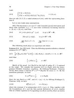
5 The singular integral equation
97
5.1 Introduction . . . . . . . . . . . . . . . . . . . . . . . . . . . . . . . . . . . . . . . . . . . . . . . . . . . 97
5.2 Abel’s problem . . . . . . . . . . . . . . . . . . . . . . . . . . . . . . . . . . . . . . . . . . . . . . . . . 98
5.3 The generalized Abel’s integral equation of the first kind . . . . . . . . . . . 99
5.4 Abel’s problem of the second kind integral equation . . . . . . . . . .. . . . . 100
5.5 The weakly-singular Volterra equation . . . . . . . . . . . . . . . . . . . . . .. . . . . 101
5.6 Equations with Cauchy’s principal value of an integral

and Hilbert’s transformation . . . . . . . . . . . . . . . . . . . . . . . . . . . . . . . . . . . . 104
5.7 Use of Hilbert transforms in signal processing . . . . . . . . . . . . . . . . . . . 114
5.8 The Fourier transform . . . . . . . . . . . . . . . . . . . . . . . . . . . . . . . . . . . . . . . . . 116
5.9 The Hilbert transform via Fourier transform . . . . . . . . . . . . . . . . .. . . . . 118
5.10 The Hilbert transform via the ±π/2 phase shift . . . . . . . . . . . . . .. . . . . 119
5.11 Properties of the Hilbert transform . . . . . . . . . . . . . . . . . . . . . . . . . . . . . . 121
5.11.1 Linearity . . . . . . . . . . . . . . . . . . . . . . . . . . . . . . . . . . . . . . . . . . . . . 121
5.11.2 Multiple Hilbert transforms and their inverses . . . . . . . . . . . . 121
5.11.3 Derivatives of the Hilbert transform . . . . . . . . . . . . . . . . . . . . . 123
5.11.4 Orthogonality properties . . . . . . . . . . . . . . . . . . . . . . . . . . . . . . . 123
5.11.5 Energy aspects of the Hilbert transform . . . . . . . . . . . . .. . . . . 124
5.12 Analytic signal in time domain . . . . . . . . . . . . . . . . . . . . . . . . . . . . . . . . . 125
5.13 Hermitian polynomials . . . . . . . . . . . . . . . . . . . . . . . . . . . . . . . . . . . . . . . . 125
5.14 The finite Hilbert transform . . . . . . . . . . . . . . . . . . . . . . . . . . . . . . . . . . . . 129
5.14.1 Inversion formula for the finite Hilbert transform . . . . . . . . . 131
5.14.2 Trigonometric series form . . . . . . . . . . . . . . . . . . . . . . . . . . . . . . 132
5.14.3 An important formula . . . . . . . . . . . . . . . . . . . . . . . . . . . . . . . . . . 133


MM-165

Prelims.tex

29/5/2007

16: 38

Page iii

5.15 Sturm–Liouville problems . . . . . . . . . . . . . . . . . . . . . . . . . . . . . . . . . . . . . 134

5.16 Principles of variations . . . . . . . . . . . . . . . . . . . . . . . . . . . . . . . . . . . . . . . . 142
5.17 Hamilton’s principles . . . . . . . . . . . . . . . . . . . . . . . . . . . . . . . . . . . . . . . . . . 146
5.18 Hamilton’s equations . . . . . . . . . . . . . . . . . . . . . . . . . . . . . . . . . . . . . . . . . . 151
5.19 Some practical problems . . . . . . . . . . . . . . . . . . . . . . . . . . . . . . . . . . . . . . . 156
5.20 Exercises . . . . . . . . . . . . . . . . . . . . . . . . . . . . . . . . . . . . . . . . . . . . . . . . . . . . . 161
References . . . . . . . . . . . . . . . . . . . . . . . . . . . . . . . . . . . . . . . . . . . . . . . . . . . . . . . . 164
6

Integro-differential equations
165
6.1 Introduction . . . . . . . . . . . . . . . . . . . . . . . . . . . . . . . . . . . . . . . . . . . . . . . . . . 165
6.2 Volterra integro-differential equations . . . . . . . . . . . . . . . . . . . . . . . . . . . 166
6.2.1 The series solution method . . . . . . . . . . . . . . . . . . . . . . . . . . . . . 166
6.2.2 The decomposition method . . . . . . . . . . . . . . . . . . . . . . . . . . . . . 169
6.2.3 Converting to Volterra integral equations . . . . . . . . . . . .. . . . . 173
6.2.4 Converting to initial value problems . . . . . . . . . . . . . . . . . . . . . 175
6.3 Fredholm integro-differential equations . . . . . . . . . . . . . . . . . . . . .. . . . . 177
6.3.1 The direct computation method . . . . . . . . . . . . . . . . . . . . . . . . . 177
6.3.2 The decomposition method . . . . . . . . . . . . . . . . . . . . . . . . . . . . . 179
6.3.3 Converting to Fredholm integral equations . . . . . . . . . . . . . . . 182
6.4 The Laplace transform method . . . . . . . . . . . . . . . . . . . . . . . . . . . . . . . . . 184
6.5 Exercises . . . . . . . . . . . . . . . . . . . . . . . . . . . . . . . . . . . . . . . . . . . . . . . . . . . . . 187
References . . . . . . . . . . . . . . . . . . . . . . . . . . . . . . . . . . . . . . . . . . . . . . . . . . . . . . . . 187

7

Symmetric kernels and orthogonal systems of functions
189
7.1 Development of Green’s function in one-dimension . . . . . . . . . . . . . . . 189
7.1.1 A distributed load of the string . . . . . . . . . . . . . . . . . . . . . . . . . . 189

7.1.2 A concentrated load of the strings . . . . . . . . . . . . . . . . . . . . . . . 190
7.1.3 Properties of Green’s function . . . . . . . . . . . . . . . . . . . . . . . . . . 194
7.2 Green’s function using the variation of parameters . . . . . . . . . . . . . . . . 200
7.3 Green’s function in two-dimensions . . . . . . . . . . . . . . . . . . . . . . . . . . . . . 207
7.3.1 Two-dimensional Green’s function . . . . . . . . . . . . . . . . . .. . . . . 208
7.3.2 Method of Green’s function . . . . . . . . . . . . . . . . . . . . . . . .. . . . . 211
7.3.3 The Laplace operator . . . . . . . . . . . . . . . . . . . . . . . . . . . . . . . . . . 211
7.3.4 The Helmholtz operator . . . . . . . . . . . . . . . . . . . . . . . . . . . . . . . . 212
7.3.5 To obtain Green’s function by the method of images . .. . . . . 219
7.3.6 Method of eigenfunctions . . . . . . . . . . . . . . . . . . . . . . . . . . . . . . 221
7.4 Green’s function in three-dimensions . . . . . . . . . . . . . . . . . . . . . . . . . . . . 223
7.4.1 Green’s function in 3D for physical problems . . . . . . . .. . . . . 226
7.4.2 Application: hydrodynamic pressure forces . . . . . . . . . .. . . . . 231
7.4.3 Derivation of Green’s function . . . . . . . . . . . . . . . . . . . . . . . . . . 232
7.5 Numerical formulation. . . . . . . . . . . . . . . . . . . . . . . . . . . . . . . . . . . .. . . . . 244
7.6 Remarks on symmetric kernel and a process
of orthogonalization . . . . . . . . . . . . . . . . . . . . . . . . . . . . . . . . . . . . . . . . . . . 249
7.7 Process of orthogonalization . . . . . . . . . . . . . . . . . . . . . . . . . . . . . . . . . . . 251


MM-165

Prelims.tex

29/5/2007

16: 38

Page iv

7.8 The problem of vibrating string: wave equation . . . . . . . . . . . . . .. . . . . 254
7.9 Vibrations of a heavy hanging cable . . . . . . . . . . . . . . . . . . . . . . . . . . . . . 256
7.10 The motion of a rotating cable . . . . . . . . . . . . . . . . . . . . . . . . . . . . . . . . . . 261
7.11 Exercises . . . . . . . . . . . . . . . . . . . . . . . . . . . . . . . . . . . . . . . . . . . . . . . . . . . . . 264
References . . . . . . . . . . . . . . . . . . . . . . . . . . . . . . . . . . . . . . . . . . . . . . . . . . . . . . . . 266
8 Applications
269
8.1 Introduction . . . . . . . . . . . . . . . . . . . . . . . . . . . . . . . . . . . . . . . . . . . . . . . . . . 269
8.2 Ocean waves . . . . . . . . . . . . . . . . . . . . . . . . . . . . . . . . . . . . . . . . . . . . .. . . . . 269
8.2.1 Introduction . . . . . . . . . . . . . . . . . . . . . . . . . . . . . . . . . . . . . . . . . . 270
8.2.2 Mathematical formulation . . . . . . . . . . . . . . . . . . . . . . . . . . . . . . 270
8.3 Nonlinear wave–wave interactions . . . . . . . . . . . . . . . . . . . . . . . . . . . . . . 273
8.4 Picard’s method of successive approximations . . . . . . . . . . . . . . .. . . . . 274
8.4.1 First approximation . . . . . . . . . . . . . . . . . . . . . . . . . . . . . . . . . . . . 274
8.4.2 Second approximation . . . . . . . . . . . . . . . . . . . . . . . . . . . . . . . . . 275
8.4.3 Third approximation . . . . . . . . . . . . . . . . . . . . . . . . . . . . . . . . . . . 276
8.5 Adomian decomposition method . . . . . . . . . . . . . . . . . . . . . . . . . . . . . . . . 278
8.6 Fourth-order Runge−Kutta method . . . . . . . . . . . . . . . . . . . . . . . . . . . . . 282
8.7 Results and discussion . . . . . . . . . . . . . . . . . . . . . . . . . . . . . . . . . . . . . . . . . 284
8.8 Green’s function method for waves . . . . . . . . . . . . . . . . . . . . . . . . .. . . . . 288
8.8.1 Introduction . . . . . . . . . . . . . . . . . . . . . . . . . . . . . . . . . . . . . . . . . . 288
8.8.2 Mathematical formulation . . . . . . . . . . . . . . . . . . . . . . . . . . . . . . 289
8.8.3 Integral equations . . . . . . . . . . . . . . . . . . . . . . . . . . . . . . . . . . . . . 292
8.8.4 Results and discussion . . . . . . . . . . . . . . . . . . . . . . . . . . . . . . . . . 296
8.9 Seismic response of dams . . . . . . . . . . . . . . . . . . . . . . . . . . . . . . . . . . . . . . 299
8.9.1 Introduction . . . . . . . . . . . . . . . . . . . . . . . . . . . . . . . . . . . . . . . . . . 299
8.9.2 Mathematical formulation . . . . . . . . . . . . . . . . . . . . . . . . . . . . . . 300
8.9.3 Solution . . . . . . . . . . . . . . . . . . . . . . . . . . . . . . . . . . . . . . . . . . . . . . 302
8.10 Transverse oscillations of a bar . . . . . . . . . . . . . . . . . . . . . . . . . . . . . . . . . 306
8.11 Flow of heat in a metal bar . . . . . . . . . . . . . . . . . . . . . . . . . . . . . . . . . . . . . 309

8.12 Exercises . . . . . . . . . . . . . . . . . . . . . . . . . . . . . . . . . . . . . . . . . . . . . . . . . . . . . 315
References . . . . . . . . . . . . . . . . . . . . . . . . . . . . . . . . . . . . . . . . . . . . . . . . . . . . . . . . 317
Appendix A

Miscellaneous results . . . . . . . . . . . . . . . . . . . . . . . . . . . . . . . . . . . 319

Appendix B Table of Laplace transforms . . . . . . . . . . . . . . . . . . . . . . . . . . . . . 327
Appendix C

Specialized Laplace inverses . . . . . . . . . . . . . . . . . . . . . . . . . . . . . 341

Answers to some selected exercises . . . . . . . . . . . . . . . . . . . . . . . . . . . . . . . . . . . . . 345
Subject index . . . . . . . . . . . . . . . . . . . . . . . . . . . . . . . . . . . . . . . . . . . . . . . . . . . . . . . . . 355


Preface

While scientists and engineers can already choose from a number of books on
integral equations, this new book encompasses recent developments including
some preliminary backgrounds of formulations of integral equations governing the
physical situation of the problems. It also contains elegant analytical and numerical
methods, and an important topic of the variational principles. This book is primarily
intended for the senior undergraduate students and beginning graduate students
of engineering and science courses. The students in mathematical and physical
sciences will find many sections of divert relevance. The book contains eight
chapters. The chapters in the book are pedagogically organized. This book is
specially designed for those who wish to understand integral equations without
having extensive mathematical background. Some knowledge of integral calculus,
ordinary differential equations, partial differential equations, Laplace transforms,
Fourier transforms, Hilbert transforms, analytic functions of complex variables and

contour integrations are expected on the part of the reader.
The book deals with linear integral equations, that is, equations involving an
unknown function which appears under an integral sign. Such equations occur
widely in diverse areas of applied mathematics and physics. They offer a powerful
technique for solving a variety of practical problems. One obvious reason for using
the integral equation rather than differential equations is that all of the conditions
specifying the initial value problems or boundary value problems for a differential
equation can often be condensed into a single integral equation. In the case of
partial differential equations, the dimension of the problem is reduced in this process
so that, for example, a boundary value problem for a partial differential equation in
two independent variables transform into an integral equation involving an unknown
function of only one variable. This reduction of what may represent a complicated
mathematical model of a physical situation into a single equation is itself a significant
step, but there are other advantages to be gained by replacing differentiation with
integration. Some of these advantages arise because integration is a smooth process,
a feature which has significant implications when approximate solutions are sought.
Whether one is looking for an exact solution to a given problem or having to settle
for an approximation to it, an integral equation formulation can often provide a
useful way forward. For this reason integral equations have attracted attention for


most of the last century and their theory is well-developed.
While I was a graduate student at the Imperial College’s mathematics department
during 1966-1969, I was fascinated with the integral equations course given by
Professor Rosenblatt. His deep knowledge about the subject impressed me and
gave me a love for integral equations. One of the aims of the course given by
Professor Rosenblatt was to bring together students from pure mathematics and
applied mathematics, often regarded by the students as totally unconnected. This
book contains some theoretical development for the pure mathematician but these
theories are illustrated by practical examples so that an applied mathematician can

easily understand and appreciate the book.
This book is meant for the senior undergraduate and the first year postgraduate
student. I assume that the reader is familiar with classical real analysis, basic linear
algebra and the rudiments of ordinary differential equation theory. In addition, some
acquaintance with functional analysis and Hilbert spaces is necessary, roughly at
the level of a first year course in the subject, although I have found that a limited
familiarity with these topics is easily considered as a bi-product of using them in the
setting of integral equations. Because of the scope of the text and emphasis on
practical issues, I hope that the book will prove useful to those working in application
areas who find that they need to know about integral equations.
I felt for many years that integral equations should be treated in the fashion of
this book and I derived much benefit from reading many integral equation books
available in the literature. Others influence in some cases by acting more in spirit,
making me aware of the sort of results we might seek, papers by many prominent
authors. Most of the material in the book has been known for many years, although
not necessarily in the form in which I have presented it, but the later chapters do
contain some results I believe to be new.
Digital computers have greatly changed the philosophy of mathematics as applied
to engineering. Many applied problems that cannot be solved explicitly by analytical
methods can be easily solved by digital computers. However, in this book I have
attempted the classical analytical procedure. There is too often a gap between the
approaches of a pure and an applied mathematician to the same problem, to the
extent that they may have little in common. I consider this book a middle road where
I develop, the general structures associated with problems which arise in applications
and also pay attention to the recovery of information of practical interest. I did not
avoid substantial matters of calculations where these are necessary to adapt the
general methods to cope with classes of integral equations which arise in the
applications. I try to avoid the rigorous analysis from the pure mathematical view
point, and I hope that the pure mathematician will also be satisfied with the dealing
of the applied problems.

The book contains eight chapters, each being divided into several sections. In
this text, we were mainly concerned with linear integral equations, mostly of secondkind. Chapter 1 introduces the classifications of integral equations and necessary
techniques to convert differential equations to integral equations or vice versa.
Chapter 2 deals with the linear Volterra integral equations and the relevant solution
techniques. Chapter 3 is concerned with the linear Fredholme integral equations


and also solution techniques. Nonlinear integral equations are investigated in
Chapter 4. Adomian decomposition method is used heavily to determine the solution
in addition to other classical solution methods. Chapter 5 deals with singular integral
equations along with the variational principles. The transform calculus plays an
important role in this chapter. Chapter 6 introduces the integro-differential equations.
The Volterra and Fredholm type integro-differential equations are successfully
manifested in this chapter. Chapter 7 contains the orthogonal systems of functions.
Green’s functions as the kernel of the integral equations are introduced using simple
practical problems. Some practical problems are solved in this chapter. Chapter 8
deals with the applied problems of advanced nature such as arising in ocean waves,
seismic response, transverse oscillations and flows of heat. The book concludes
with four appendices.
In this computer age, classical mathematics may sometimes appear irrelevant.
However, use of computer solutions without real understanding of the underlying
mathematics may easily lead to gross errors. A solid understanding of the relevant
mathematics is absolutely necessary. The central topic of this book is integral
equations and the calculus of variations to physical problems. The solution
techniques of integral equations by analytical procedures are highlighted with many
practical examples.
For many years the subject of functional equations has held a prominent place in
the attention of mathematicians. In more recent years this attention has been directed
to a particular kind of functional equation, an integral equation, wherein the unknown
function occurs under the integral sign. The study of this kind of equation is

sometimes referred to as the inversion of a definite integral.
In the present book I have tried to present in readable and systematic manner the
general theory of linear integral equations with some of its applications. The
applications given are to differential equations, calculus of variations, and some
problems which lead to differential equations with boundary conditions. The
applications of mathematical physics herein given are to Neumann’s problem and
certain vibration problems which lead to differential equations with boundary
conditions. An attempt has been made to present the subject matter in such a way
as to make the book suitable as a text on this subject in universities.
The aim of the book is to present a clear and well-organized treatment of the
concept behind the development of mathematics and solution techniques. The text
material of this book is presented in a highly readable, mathematically solid format.
Many practical problems are illustrated displaying a wide variety of solution
techniques.
There are more than 100 solved problems in this book and special attention is
paid to the derivation of most of the results in detail, in order to reduce possible
frustrations to those who are still acquiring the requisite skills. The book contains
approximately 150 exercises. Many of these involve extension of the topics presented
in the text. Hints are given in many of these exercises and answers to some selected
exercises are provided in Appendix C. The prerequisites to understand the material
contained in this book are advanced calculus, vector analysis and techniques of
solving elementary differential equations. Any senior undergraduate student who


has spent three years in university, will be able to follow the material contained in
this book. At the end of most of the chapters there are many exercises of practical
interest demanding varying levels of effort.
While it has been a joy to write this book over a number of years, the fruits of this
labor will hopefully be in learning of the enjoyment and benefits realized by the
reader. Thus the author welcomes any suggestions for the improvement of the text.

M. Rahman
2007


Acknowledgements

The author is immensely grateful to the Natural Sciences and Engineering Research
Council of Canada (NSERC) for its financial support. Mr. Adhi Susilo deserves my
appreciation in assisting me in the final drafting of the figures of this book for
publication. The author is thankful to Professor Carlos Brebbia, Director of Wessex
Institute of Technology (WIT) for his kind advice and interest in the contents of the
book. I am also grateful to the staff of WIT Press, Southampton, UK for their superb
job in producing this manuscript in an excellent book form.


This page intentionally left blank


MM-165

1

CH001.tex

26/4/2007

13: 43

Page 1

Introduction

1.1 Preliminary concept of the integral equation
An integral equation is defined as an equation in which the unknown function u(x)
to be determined appear under the integral sign. The subject of integral equations is
one of the most useful mathematical tools in both pure and applied mathematics. It
has enormous applications in many physical problems. Many initial and boundary
value problems associated with ordinary differential equation (ODE) and partial
differential equation (PDE) can be transformed into problems of solving some
approximate integral equations (Refs. [2], [3] and [6]).
The development of science has led to the formation of many physical laws,
which, when restated in mathematical form, often appear as differential equations.
Engineering problems can be mathematically described by differential equations,
and thus differential equations play very important roles in the solution of practical problems. For example, Newton’s law, stating that the rate of change of the
momentum of a particle is equal to the force acting on it, can be translated into
mathematical language as a differential equation. Similarly, problems arising in
electric circuits, chemical kinetics, and transfer of heat in a medium can all be
represented mathematically as differential equations.
A typical form of an integral equation in u(x) is of the form
β(x)

u(x) = f (x) + λ

K(x, t)u(t)dt

(1.1)

α(x)

where K(x, t) is called the kernel of the integral equation (1.1), and α(x) and β(x) are

the limits of integration. It can be easily observed that the unknown function u(x)
appears under the integral sign. It is to be noted here that both the kernel K(x, t)
and the function f (x) in equation (1.1) are given functions; and λ is a constant
parameter. The prime objective of this text is to determine the unknown function
u(x) that will satisfy equation (1.1) using a number of solution techniques. We
shall devote considerable efforts in exploring these methods to find solutions of the
unknown function.
1


MM-165

CH001.tex

26/4/2007

13: 43

Page 2

2 Integral Equations and their Applications

1.2 Historical background of the integral equation
In 1825 Abel, an Italian mathematician, first produced an integral equation in connection with the famous tautochrone problem (see Refs. [1], [4] and [5]). The
problem is connected with the determination of a curve along which a heavy particle, sliding without friction, descends to its lowest position, or more generally,
such that the time of descent is a given function of its initial position. To be more
specific, let us consider a smooth curve situated in a vertical plane. A heavy particle
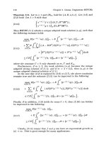
starts from rest at any position P (see Figure 1.1).
Let us find, under the action of gravity, the time T of descent to the lowest
position O. Choosing O as the origin of the coordinates, the x-axis vertically upward,

and the y-axis horizontal. Let the coordinates of P be (x, y), of Q be (ξ, η), and s
the arc OQ.
At any instant, the particle will attain the potential energy and kinetic energy at
Q such that the sum of which is constant, and mathematically it can be stated as
K.E. + P.E. = constant
2
1
2 mv + mgξ
or 12 v2 + gξ

= constant
=C

(1.2)

where m is the mass of the particle, v(t) the speed of the particle at Q, g the
acceleration due to gravity, and ξ the vertical coordinate of the particle at Q. Initially, v(0) = 0 at P, the vertical coordinate is x, and hence the constant C can be
determined as C = gx.
Thus, we have
1 2
2v

+ gξ = gx
v2 = 2g(x − ξ)
v = ± 2g(x − ξ)

x

(1.3)

P(x, y)

Q(ξ, η)

s
O

y

Figure 1.1: Schematic diagram of a smooth curve.


MM-165

CH001.tex

26/4/2007

13: 43

Page 3

Introduction

3

But v = ds
dt = speed along the curve s. Therefore,
ds
= ± 2g(x − ξ).

dt
Considering the negative value of
variables, we obtain
Q

ds
dt

and integrating from P to Q by separating the

Q

dt = −

P

ds
2g(x − ξ)

P
Q

t=−

ds
2g(x − ξ)

P

The total time of descent is, then,

O

O

dt = −

P

P
P

T =

O

ds
2g(x − ξ)
ds
2g(x − ξ)

(1.4)

If the shape of the curve is given, then s can be expressed in terms of ξ and hence ds
can be expressed in terms of ξ. Let ds = u(ξ)dξ, the equation (1.4) takes the form
x

T =

u(ξ)dξ
2g(x − ξ)

0

Abel set himself the problem of finding the curve for which the time T of descent is
a given function of x, say f (x). Our problem, then, is to find the unknown function
u(x) from the equation
x

f (x) =

u(ξ)dξ
2g(x − ξ)

0
x

=

K(x, ξ)u(ξ)dξ.

(1.5)

0

This is a linear integral equation of the first kind for the determination of u(x).
Here, K(x, ξ) = √ 1
is the kernel of the integral equation. Abel solved this
2g(x − ξ)

problem already in 1825, and in essentially the same manner which we shall use;

however, he did not realize the general importance of such types of functional
equations.


MM-165

CH001.tex

26/4/2007

13: 43

Page 4

4 Integral Equations and their Applications

1.3 An illustration from mechanics
The differential equation which governs the mass-spring system is given by (see
Figure 1.2)
m

d 2u
+ ku = f (t) (0 ≤ t < ∞)
dt 2

with the initial conditions, u(0) = u0 , and du
dt = u˙0 , where k is the stiffness of the
string, f (t) the prescribed applied force, u0 the initial displacement, and u˙0 the
initial value. This problem can be easily solved by using the Laplace transform. We
transform this ODE problem into an equivalent integral equation as follows:

Integrating the ODE with respect to t from 0 to t yields
m

du
− mu˙0 + k
dt

t

t

u(τ)dτ =

f (τ)dτ.

0

0

Integrating again gives
t

mu(t) − mu0 − mu0 t + k
0
t

t

t

u(τ)dτdτ =

0

t

f (τ)dτdτ.
0

(1.6)

0

t

t

t

We know that if y(t) = 0 0 u(τ)dτdτ, then L{y(t)} = L{ 0 0 f (τ)dτdτ} =
1
L{u(t)}.
Therefore, by using the convolution theorem, the Laplace inverse is
2
s
t
obtained as y(t) = 0 (t − τ)u(τ)dτ, which is known as the convolution integral.
Hence using the convolution property, equation (1.6) can be written as
u(t) = u0 + u˙0 t +

1
m

t

(t − τ)f (τ)dτ −

0

k
m

t

(t − τ)u(τ)dτ,

(1.7)

0

which is an integral equation. Unfortunately, this is not the solution of the original
problem, because the presence of the unknown function u(t) under the integral
sign. Rather, it is an example of an integral equation because of the presence of
the unknown function within the integral. Beginning with the integral equation, it
is possible to reverse our steps with the help of the Leibnitz rule, and recover the
original system, so that they are equivalent. In the present illustration, the physics
(namely, Newton’s second law ) gave us the differential equation of motion, and it
u(t)

m

f(t)

k

Figure 1.2: Mass spring system.


MM-165

CH001.tex

26/4/2007

13: 43

Page 5

Introduction

5

was only by manipulation, we obtained the integral equation. In the Abel’s problem,
the physics gave us the integral equation directly. In any event, observe that we
can solve the integral equation by application of the Laplace Transform. Integral
equations of the convolution type can easily be solved by the Laplace transform .

1.4 Classification of integral equations
An integral equation can be classified as a linear or nonlinear integral equation as we
have seen in the ordinary and partial differential equations. In the previous section,

we have noticed that the differential equation can be equivalently represented by
the integral equation. Therefore, there is a good relationship between these two
equations.
The most frequently used integral equations fall under two major classes, namely
Volterra and Fredholm integral equations. Of course, we have to classify them as
homogeneous or nonhomogeneous; and also linear or nonlinear. In some practical
problems, we come across singular equations also.
In this text, we shall distinguish four major types of integral equations – the
two main classes and two related types of integral equations. In particular, the four
types are given below:
•
•
•
•

Volterra integral equations
Fredholm integral equations
Integro-differential equations
Singular integral equations

We shall outline these equations using basic definitions and properties of each type.
1.4.1 Volterra integral equations
The most standard form of Volterra linear integral equations is of the form
x

φ(x)u(x) = f (x) + λ

K(x, t)u(t)dt

(1.8)

a

where the limits of integration are function of x and the unknown function u(x)
appears linearly under the integral sign. If the function φ(x) = 1, then equation
(1.8) simply becomes
x

u(x) = f (x) + λ

K(x, t)u(t)dt

(1.9)

a

and this equation is known as the Volterra integral equation of the second kind;
whereas if φ(x) = 0, then equation (1.8) becomes
x

f (x) + λ

K(x, t)u(t)dt = 0

a

which is known as the Volterra equation of the first kind.

(1.10)

MM-165

CH001.tex

26/4/2007

13: 43

Page 6

6 Integral Equations and their Applications
1.4.2 Fredholm integral equations
The most standard form of Fredholm linear integral equations is given by the form
b

φ(x)u(x) = f (x) + λ

K(x, t)u(t)dt

(1.11)

a

where the limits of integration a and b are constants and the unknown function
u(x) appears linearly under the integral sign. If the function φ(x) = 1, then (1.11)
becomes simply
b

u(x) = f (x) + λ

K(x, t)u(t)dt

(1.12)

a

and this equation is called Fredholm integral equation of second kind; whereas if
φ(x) = 0, then (1.11) yields
b

f (x) + λ

K(x, t)u(t)dt = 0

(1.13)

a

which is called Fredholm integral equation of the first kind.
Remark
It is important to note that integral equations arise in engineering, physics, chemistry, and biological problems. Many initial and boundary value problems associated
with the ordinary and partial differential equations can be cast into the integral
equations of Volterra and Fredholm types, respectively.
If the unknown function u(x) appearing under the integral sign is given in
the functional form F(u(x)) such as the power of u(x) is no longer unity, e.g.
F(u(x)) = un (x), n = 1, or sin u(x) etc., then theVolterra and Fredholm integral equations are classified as nonlinear integral equations. As for examples, the following
integral equations are nonlinear integral equations:
x

u(x) = f (x) + λ

K(x, t) u2 (t) dt

a
x

u(x) = f (x) + λ

K(x, t) sin (u(t)) dt
a
x

u(x) = f (x) + λ

K(x, t) ln (u(t)) dt
a

Next, if we set f (x) = 0, in Volterra or Fredholm integral equations, then the resulting equation is called a homogeneous integral equation, otherwise it is called
nonhomogeneous integral equation.


MM-165

CH001.tex

26/4/2007

13: 43

Page 7

Introduction

7

1.4.3 Singular integral equations
A singular integral equation is defined as an integral with the infinite limits or when
the kernel of the integral becomes unbounded at a certain point in the interval. As
for examples,
u(x) = f (x) + λ
x

f (x) =

∞
−∞

u(t)dt

1
u(t)dt, 0 < α < 1
(x − t)α

0

(1.14)

are classified as the singular integral equations.
1.4.4 Integro-differential equations

In the early 1900, Vito Volterra studied the phenomenon of population growth, and
new types of equations have been developed and termed as the integro-differential
equations. In this type of equations, the unknown function u(x) appears as the
combination of the ordinary derivative and under the integral sign. In the electrical
engineering problem, the current I (t) flowing in a closed circuit can be obtained in
the form of the following integro-differential equation,
L

dI
1
+ RI +
dt
C

t

I (τ)dτ = f (t),

I (0) = I0

(1.15)

0

where L is the inductance, R the resistance, C the capacitance, and f (t) the applied
voltage. Similar examples can be cited as follows:
x

u (x) = f (x) + λ

(x − t)u(t)dt, u(0) = 0, u (0) = 1,

(1.16)

(xt)u(t)dt, u(0) = 1.

(1.17)

0
1

u (x) = f (x) + λ
0

Equations (1.15) and (1.16) are of Volterra type integro-differential equations,
whereas equation (1.17) Fredholm type integro-differential equations. These
terminologies were concluded because of the presence of indefinite and definite
integrals.

1.5 Converting Volterra equation to ODE
In this section, we shall present the technique that converts Volterra integral equations of second kind to equivalent ordinary differential equations. This may be


MM-165

CH001.tex

26/4/2007

13: 43

Page 8

8 Integral Equations and their Applications
achieved by using the Leibnitz rule of differentiating the integral
with respect to x, we obtain
d
dx

b(x)

b(x)

F(x, t)dt =

a(x)

a(x)

−

b(x)
a(x) F(x, t)dt

db(x)
∂F(x, t)
dt +
F(x, b(x))
∂x
dx

da(x)
F(x, a(x)),
dx

(1.18)

where F(x, t) and ∂F
∂x (x, t) are continuous functions of x and t in the domain
α ≤ x ≤ β and t0 ≤ t ≤ t1 ; and the limits of integration a(x) and b(x) are defined
functions having continuous derivatives for α ≤ x ≤ β. For more information the
reader should consult the standard calculus book including Rahman (2000). A
simple illustration is presented below:
d
dx

x

x

sin(x − t)u(t)dt =

0

cos(x − t)u(t)dt +

0

d0
(sin(x − 0)u(0))

dx

−
x

=

dx
(sin(x − x)u(x))
dx

cos(x − t)u(t)dt.

0

1.6 Converting IVP to Volterra equations
We demonstrate in this section how an initial value problem (IVP) can be transformed to an equivalent Volterra integral equation. Let us consider the integral
equation
t

y(t) =

f (t)dt

(1.19)

0

The Laplace transform of f (t) is defined as L{f (t)} =
this definition, equation (1.19) can be transformed to

∞ −st
f (t)dt = F(s).
0 e

1
L{y(t)} = L{f (t)}.
s
In a similar manner, if y(t) =

t t
0 0

f (t)dtdt, then

L{y(t)} =

1
L{f (t)}.
s2

This can be inverted by using the convolution theorem to yield
t

y(t) =
0

(t − τ)f (τ)dτ.

Using

MM-165

CH001.tex

26/4/2007

13: 43

Page 9

Introduction

9

If
t

y(t) =
0

t

t

···

0

f (t)dtdt · · · dt

0
n-fold

integrals

then L{y(t)} = s1n L{f (t)}. Using the convolution theorem, we get the Laplace
inverse as
t

y(t) =
0

(t − τ)n−1
f (τ)dτ.
(n − 1)!

Thus the n-fold integrals can be expressed as a single integral in the following
manner:
t
0

t
0

t

···
0

n-fold

t

f (t)dtdt · · · dt =
0

(t − τ)n−1
f (τ)dτ.
(n − 1)!

(1.20)

integrals

This is an essential and useful formula that has enormous applications in the
integral equation problems.

1.7 Converting BVP to Fredholm integral equations
In the last section we have demonstrated how an IVP can be transformed to an
equivalent Volterra integral equation. We present in this section how a boundary
value problem (BVP) can be converted to an equivalent Fredholm integral equation.
The method is similar to that discussed in the previous section with some exceptions
that are related to the boundary conditions. It is to be noted here that the method
of reducing a BVP to a Fredholm integral equation is complicated and rarely used.
We demonstrate this method with an illustration.
Example 1.1
Let us consider the following second-order ordinary differential with the given
boundary conditions.

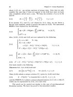
y (x) + P(x)y (x) + Q(x)y(x) = f (x)

(1.21)

with the boundary conditions
x=a:

y(a) = α

y=b:

y(b) = β

(1.22)

where α and β are given constants. Let us make transformation
y (x) = u(x)

(1.23)


MM-165

CH001.tex

26/4/2007

13: 43

Page 10

10 Integral Equations and their Applications
Integrating both sides of equation (1.23) from a to x yields
x

y (x) = y (a) +

u(t)dt

(1.24)

a

Note that y (a) is not prescribed yet. Integrating both sides of equation (1.24) with
respect to x from a to x and applying the given boundary condition at x = a, we find
x

y(x) = y(a) + (x − a)y (a) +

x

u(t)dtdt
a

a

x

= α + (x − a)y (a) +

x

u(t)dtdt
a

(1.25)

a

and using the boundary condition at x = b yields
b

y(b) = β = α + (b − a)y (a) +

b

u(t)dtdt,
a

a

and the unknown constant y (a) is determined as
y (a) =

1
β−α
−
b−a
b−a

b

b

u(t)dtdt.
a

(1.26)

a

Hence the solution (1.25) can be rewritten as
y(x) = α + (x − a)
x

+

1
β−α
−
b−a
b−a

b

b

u(t)dtdt
a

a

x

u(t)dtdt
a

(1.27)

a

Therefore, equation (1.21) can be written in terms of u(x) as
x

u(x) = f (x) − P(x) y (a) +

u(t)dt
a
x

−Q(x) α + (x − a)y (a) +

x

u(t)dtdt
a

(1.28)

a

where u(x) = y (x) and so y(x) can be determined, in principle, from equation (1.27).
This is a complicated procedure to determine the solution of a BVP by equivalent
Fredholm integral equation.