Dynamic modelling of biomass gasification in a cocurrent fixed bed gasifier
Bạn đang xem bản rút gọn của tài liệu. Xem và tải ngay bản đầy đủ của tài liệu tại đây (2.54 MB, 13 trang )
Energy Conversion and Management xxx (2016) xxx–xxx
Contents lists available at ScienceDirect
Energy Conversion and Management
journal homepage: www.elsevier.com/locate/enconman
Dynamic modelling of biomass gasification in a co-current fixed bed
gasifier
Robert Mikulandric´ a,b,⇑, Dorith Böhning c, Rene Böhme c, Lieve Helsen d, Michael Beckmann c,
Drazˇen Loncˇar a
a
Department of Energy, Power Engineering and Ecology, Faculty of Mechanical Engineering and Naval Architecture, University of Zagreb, No. 5 Ivana Lucˇic´a, 10002 Zagreb, Croatia
Department of Biosystems, Faculty of Bioscience Engineering, KU Leuven, No. 30 Kasteelpark Arenberg, 3001 Leuven, Belgium
Institute of Power Engineering, Faculty of Mechanical Science and Engineering, Technical University Dresden, No. 3b George-Bähr-Strasse, 01069 Dresden, Germany
d
Department of Mechanical Engineering, Faculty of Engineering Science, KU Leuven, No. 300 Celestijnenlaan, 3001 Leuven, Belgium
b
c
a r t i c l e
i n f o
Article history:
Received 13 November 2015
Received in revised form 5 April 2016
Accepted 19 April 2016
Available online xxxx
Keywords:
Biomass gasification
Dynamic modelling
Artificial neural networks
Fixed bed gasifiers
a b s t r a c t
Existing technical issues related to biomass gasification process efficiency and environmental standards
are preventing the technology to become more economically viable. In order to tackle those issues a lot of
attention has been given to biomass gasification process predictive modelling. These models should be
robust enough to predict process parameters during variable operating conditions. This could be accomplished either by changes of model input variables or by changes in model structure. This paper analyses
the potential of neural network based modelling to predict process parameters during plant operation
with variable operating conditions. Dynamic neural network based model for gasification purposes will
be developed and its performance will be analysed based on measured data derived from a fixed bed biomass gasification plant operated by Technical University Dresden (TU Dresden). Dynamic neural network
can predict process temperature with an average error less than 10% and in those terms performs better
than multiple linear regression models. Average prediction error of syngas quality is lower than 30%.
Developed model is applicable for online analysis of biomass gasification process under variable operating conditions. The model is automatically modified when new operating conditions occur.
Ó 2016 Published by Elsevier Ltd.
1. Introduction
The process of biomass gasification is a high-temperature partial oxidation process in which a solid carbon based feedstock is
converted into a gaseous mixture (H2, CO, CO2, CH4, light hydrocarbons, tar, char, ash and minor contaminants) called ‘raw syngas’,
using gasifying agents [1]. Gasification products are mostly used
for separate or combined heat and power generation [2], for hydrogen production [3], methanol production [4] and production of
other chemical products [5]. A more detailed overview of available
biomass gasification technologies is published by Kirkels and
Verbong [5].
Although, gasification is a relatively well known technology, the
share of gasification in overall energy demand is small due to
current barriers concerning biomass harvesting and storage [6],
⇑ Corresponding author at: Department of Biosystems, Faculty of Bioscience
Engineering, KU Leuven, No. 30 Kasteelpark Arenberg, 3001 Leuven, Belgium.
E-mail addresses: (R. Mikulandric´),
(D. Böhning), (L. Helsen), michael.beckmann@
tu-dresden.de (M. Beckmann).
biomass pre-treatment (drying, grinding and densification), gas
cleaning (physical, thermal or catalytic), process efficiency and
syngas quality issues [7]. The performance of biomass gasification
processes is influenced by a large number of operational parameters, among them: biomass quality, fuel and air flow rate, composition and moisture content of the biomass, gasifier design,
reaction/residence time, gasifying agent, biomass particle sizes,
gasification temperature and pressure [8]. Process temperature is
considered as one of the most important process parameters which
influences syngas quality, reaction rate and tar concentration [9].
Furthermore, gasification operating conditions have tendency to
change during a long term facility operation due to ash sintering,
agglomeration and deposition on reactor walls which could cause
bed sintering and defluidisation [10].
To improve process efficiency or to guarantee constant process
quality during operation, plant operation simulation models that
enable parameter prediction as a function of various operating
conditions, are needed. Large scale experiments could be used for
this purpose on pilot plants [11] or laboratory scale setups [12]
but they are often too expensive or problematic in terms of safety.
Most of the available models for biomass gasification simulation
/>0196-8904/Ó 2016 Published by Elsevier Ltd.
Please cite this article in press as: Mikulandric´ R et al. Dynamic modelling of biomass gasification in a co-current fixed bed gasifier. Energy Convers Manage
(2016), />
R. Mikulandric´ et al. / Energy Conversion and Management xxx (2016) xxx–xxx
2
Nomenclature
Main symbols
mair
air flow rate, m3/h
mairav
average air flow rate, m3/h
mb
biomass flow rate, kg/h
mbav
average biomass flow rate, kg/h
mbfreq
fuel injection frequency, –
errorav
average error, –
b1À10
regression coefficients, –
i
measurement number, –
N
number of measurement samples, –
T
temperature, °C
t
time
are based on equilibrium models for Gibbs free energy minimisation [13], CFD analysis [14] or kinetic reactions [15]. A more
detailed review of available models for biomass gasification
process can be found in the research done by Baruah and Baruah
[16] or in comparative analysis performed by Mikulandric et al.
[17]. From this point of the state of the art, it can be concluded that
the most of available models are well capable to describe
stationary process behaviour under constant operating conditions but they are not suitable for on-line process analysis where
process dynamics under changeable operating conditions is
considered.
Adaptable/evolutionary models and optimisation methods have
potential to become a powerful methodology for gasification systems analysis, control and optimisation [18]. Artificial intelligence
systems (such as neural networks) are widely accepted as a technology that is able to deal with non-linear problems, and once
trained can perform prediction and generalisation at high speed.
Artificial neural network (ANN) based prediction models use a
non-physical modelling approach which correlates the input and
output data to develop a process prediction model. ANN is a universal function approximator that has the ability to approximate
any continuous function to an arbitrary precision even without a
priori knowledge about the structure of the function that is
approximated [19]. Dynamic neural networks with feedforward
or recurrent feedback connections are used for systems with large
delays like activated sludge processes [20], vapour-compression
liquid chillers [21], chemical process systems [22] or energy
related prediction processes [23]. Once trained ANN can predict
process parameters in circulating and bubbling fluidised bed gasifiers [24], fluidised bed gasifiers with steam as gasifying agent [25]
or in fixed bed gasifiers [26] with reasonable speed and accuracy.
However, the prediction quality of trained ANN is highly dependent on the quantity and quality of training data related to the process. Changing process operating conditions can cause large
prediction errors if the ANN models have not been modified for
those particular conditions. The importance of dynamic modelling
has been elaborated for the case of flexible operation and optimisation of carbon dioxide capture plants [27]. To encounter issues
related to changeable operating conditions and to obtain reasonable model prediction accuracy Wang and Hu [28] proposed a
dynamic parameter estimation approach using genetic algorithms
to predict thermal behaviour of buildings with changeable thermal
capacitance. For prediction of the lead-acid battery state of charge
during operation Fendri and Chaabene [29] proposed dynamic
recursive estimation Kalman filter algorithms. However, performance of a dynamic modelling approach for changeable operating
conditions in biomass gasification has still not been analysed.
Abbreviations
ANN
artificial neural networks
APE
average prediction error
CH4
methane
CO
carbon monoxide
carbon dioxide
CO2
H2
hydrogen
MFB
mean fractional bias
MLR
multiple linear regression
NMBF
normalised mean bias factor
NNM
neural network model
O2
oxygen
coefficient of determination
R2
RMSE
root mean square error
In this paper a dynamic ANN based modelling approach will be
utilised to describe the process behaviour in a 75 kWth fixed bed
gasifier, operated by TU Dresden. The ANN model needs to be able
to predict process parameters with reasonable speed and accuracy
in a gasification process with large delays and changing operating
conditions. In order to guarantee prediction accuracy for changing
operating conditions a dynamic modelling approach with automatic ANN re-training sessions will be utilised and its performance
will be compared with a dynamic multiple linear regression based
model. Reasonable prediction speed is required in order to enable
on-line parameter prediction for process analysis. Model performance has been analysed using statistical error analysis.
2. Gasification plant and operating conditions
In order to develop a neural network based model (NNM), the
neural network has to be trained using observed/measured data
to predict process parameters. Neural network based models generally require a large number of measurement data to form input
and output data sets for neural network training. Results from
NNM could differ significant if different sets of input and output
data have been used for training purposes. Due to their nature
NNMs are used to describe particular processes that occur in the
observed system during stable operating conditions. However, if
something changes in the process due to changes in operating conditions, design changes, biomass quality or other unexpected process variables the NNM structure has to be modified (NNM has to
be re-trained) to preserve prediction quality for this particular condition. For the purpose of NNM modelling 2 sets of experiments (9
experiments in total), with different operating conditions, were
conducted to form a database for NNM training. The object of modelling is a co-current fixed bed gasifier with thermal input of
75 kWth, located in Pirna (Germany), operated by TU Dresden. Biomass wood chips, distributed from a local provider, are used as fuel
in the gasification process. The facility scheme is presented in
Fig. 1.
During facility operation the biomass is firstly injected manually in a small storage room with a manually controlled valve. Once
the valve opens, the whole amount of biomass from the storage
room is injected into the biomass shredder and consequently
injected into the gasification reactor. Gasification air is distributed
by fans and injected in the process from the upper side of the gasifier, leading to a co-current flow system. Ash is removed manually
by opening ash removal valves. The biomass quality could be
determined offline by dedicated laboratory tests, however it is hard
to determine biomass quality for modelling purposes online due to
variability between batches of distributed wood chips.
Please cite this article in press as: Mikulandric´ R et al. Dynamic modelling of biomass gasification in a co-current fixed bed gasifier. Energy Convers Manage
(2016), />
R. Mikulandric´ et al. / Energy Conversion and Management xxx (2016) xxx–xxx
3
Table 1
Measurement methodology and equipment.
Process parameter
Measurement methodology and equipment
Biomass mass flow rate
Air volume flow rate
Manual weight measurement
Pressure difference based methodology (orifice
plate)
Measurement based on thermoelectric effect
(thermocouple type K)
CO, CH4, CO2 – non dispersive infrared
Absorption methodology
H2 – thermal conductivity methodology
O2 – electrochemical process
(Emerson – MLT 2 multi-component gas
analyzer)
Measurement based on platinum resistance
effect (Pt 100)
Wheatstone bridge circuit based measurement
methodology (Piezoresistive strain gauge)
Syngas temperature at the
exit of the gasifier
Syngas composition
Temperature of inlet air
Pressure in the reactor
Z
mairav ¼
Fig. 1. Scheme of co-current fixed bed biomass gasification facility operated by TU
Dresden.
Two sets of experiments were performed to analyse the process
behaviour. The first set of 4 experiments (Experiments 1–4) were
performed in 2006 and resulted in more than 40 h of operation.
The second set of 5 experiments (Experiments 5–9) were performed in 2013 and resulted in more than 35 h of operation. Experiments were performed to determine/measure following process
parameters: biomass mass flow rate (mb); air volume flow rate
(mair); syngas temperature at the exit of the gasifier; syngas composition; pressure in the reactor and temperature of inlet air. All
data was recorded on a 30 s base in accordance with relevant international standards for this type of measurements. The measurement equipment for dedicated tests is listed in Table 1.
After measurements, the data was analysed in order to define a
set of input and output datasets for NNM training after which the
data was pre-processed. For the process temperature prediction
the average biomass fuel flow rate was averaged on 25 min basis,
together with the air flow rate (Eqs. (1) and (2)). Injection frequency (the time from the last fuel injection) was also calculated
to incorporate the dynamic behaviour (delays) of the process
(instead of using a dynamic neural network modelling approach).
A detailed description of the data analysis and motivation for this
particular data analysis approach are presented in [26]. Results of
data analysis for fuel flow rate, air flow rate and fuel injection frequency for Experiments 1–4 (2006) and 5–8 (2013) are presented
in Figs. 2–4.
Z
mbav ¼
t¼i
mb dt
t¼iÀ25
ð1Þ
t¼i
mair dt
ð2Þ
t¼iÀ25
During Experiments 1–4 the amount of the injected biomass
(fuel) is in general less than during Experiments 5–8. This could
be due to different biomass quality, plant ageing, ash agglomeration or due to some other unwanted changes in the gasifier. Furthermore, the profile of the fuel flow rate has been changed.
While in Experiments 1–4 the fuel injection rate is quite constant
(can be seen from time without fuel injection diagrams) in Experiments 5–8 the fuel injection rate is more scattered during gasifier
operation and can reach up to 20 min without fuel injection (while
in Experiments 1–4 the time without fuel injection is generally less
than 7 min). Generally, more fuel in a more dispersed way has been
injected during Experiments 5–8 in comparison to Experiments 1–
4. Air injection rate profiles are rather constant in all experiments
and range between 10 and 15 m3/h. It is reasonable to assume that
due to changes in fuel flow rate and fuel injection frequency the
process will behave in a different way which will result in different
temperature profiles (together with other process parameters).
3. Modelling methods
For modelling purposes data collected from Experiments 1–9
has been used to form a database for NNM training. For artificial
neural-network (ANN) based prediction models the adaptive
network-based fuzzy inference system (ANFIS) with Suggeno type
of fuzzy model and hybrid learning algorithms with 27 nodes
(together with membership functions) in structure layers were
used. The individual Multi Input Single Output system comprises
of 4 inputs (fuel flow rate, fuel injection frequency, air flow rate
and current temperature of syngas at outlet) and one output which
represents the temperature change. A simple analysis for different
number of iterations for NNM training has been performed with
10, 25, 50 and 100 iterations. The prediction quality after 50 iterations did not improve considerably so due to a shorter computational time and to reduce the risk of NNM overfitting the NNM
model with 50 iterations has been chosen. The change in syngas
outlet temperature (to be considered as process temperature in
the further text) was set as model output. Syngas temperature
was then determined by integration of predicted temperature
changes. With this approach the process dynamics related to process temperature can be described in a qualitative way [26].
Dynamic neural network models with feedforward or recurrent
feedback connections could be used for the same purpose but
due to limitations of this approach in terms of automatic on-line
analysis in MATLAB software, a general scheme that is presented
in Fig. 5 has been used.
Please cite this article in press as: Mikulandric´ R et al. Dynamic modelling of biomass gasification in a co-current fixed bed gasifier. Energy Convers Manage
(2016), />
R. Mikulandric´ et al. / Energy Conversion and Management xxx (2016) xxx–xxx
4
Fuel flow [kg/h]
Experiment 1
Experiment 2
600
600
600
500
500
500
500
400
400
400
400
300
300
300
300
200
200
200
200
100
100
100
100
0
0
200
400
600
800
0
0
Experiment 5
Fuel flow [kg/h]
Experiment 4
Experiment 3
600
200
400
0
0
600
200
Experiment 6
400
0
0
600
600
600
600
500
500
500
500
400
400
400
400
300
300
300
300
200
200
200
200
100
100
100
100
100
200
300
400
500
0
0
100
Time [min]
200
300
400
0
0
100
Time [min]
200
300
200
300
400
Experiment 8
600
0
0
100
Experiment 7
0
0
400
100
Time [min]
200
300
400
500
Time [min]
Fig. 2. Average fuel flow rate for Experiments 1–8.
Air flow [m3/h]
Experiment 1
Experiment 2
Experiment 4
20
20
20
15
15
15
15
10
10
10
10
5
5
5
5
0
0
200
400
600
800
0
0
Experiment 5
Air flow [m3/h]
Experiment 3
20
200
400
0
0
600
Experiment 6
200
400
600
0
0
20
20
20
15
15
15
15
10
10
10
10
5
5
5
5
100
200
300
Time [min]
400
500
0
0
100
200
300
Time [min]
400
0
0
100
200
Time [min]
300
200
300
400
Experiment 8
20
0
0
100
Experiment 7
400
0
0
100
200
300
400
500
Time [min]
Fig. 3. Average air flow rate for Experiments 1–8.
The NNM model was initially trained on data derived from
Experiments 1–4. Detailed training results can be found in [26].
For the trained cases, the ANN temperature prediction model shows
good correlation with measured data [26]. After the model was initially developed based on data from Experiments 1–4 it has been
applied to predict process temperature for Experiments 5–9. As
discussed in the previous section, the process conditions in
Experiments 5–9 have changed considerably in comparison with
the conditions from Experiments 1–4 due to unknown reasons.
Therefore it is shown later in the paper that the developed NNM
has larger prediction errors than in the cases from Experiments 1–4.
A similar methodology has been applied to predict gas composition (H2, CH4 and CO) during operation. The combination of fuel
flow rate, fuel injection frequency, air flow rate and current temperature of syngas at outlet as input for NNM provided the best
prediction results in the previous study [26] and therefore those
inputs were considered again for the development of a dynamic
model for syngas composition prediction.
Please cite this article in press as: Mikulandric´ R et al. Dynamic modelling of biomass gasification in a co-current fixed bed gasifier. Energy Convers Manage
(2016), />
R. Mikulandric´ et al. / Energy Conversion and Management xxx (2016) xxx–xxx
Experiment 2
Time without fuel injection [min]
Experiment 1
Experiment 3
Experiment 4
50
50
50
50
40
40
40
40
30
30
30
30
20
20
20
20
10
10
10
10
0
0
200
400
600
800
0
0
Experiment 5
Time without fuel injection [min]
5
200
400
0
0
600
Experiment 6
200
400
600
0
0
50
50
50
40
40
40
40
30
30
30
30
20
20
20
20
10
10
10
10
100
200 300
Time [min]
400
500
0
0
100
200
300
Time [min]
400
0
0
100
200
300
Time [min]
200
300
400
Experiment 8
50
0
0
100
Experiment 7
400
0
0
100
200 300
Time [min]
400
500
Fig. 4. Time without fuel injection for Experiments 1–8.
For additional model performance analysis, temperature predictions from developed NNM have been compared to temperature
predictions of Multiple Linear Regression (MLR) models. 2 different
MLR models have been utilised for analysis. General form of first
(MLR1) model is given in Eq. (5) while general form of second
(MLR2) model is given in Eq. (6). During analysis MLR models will
follow the same procedure for model re-training as for NNMs. Similar analysis approach can be found in the research performed by
Vlachogianni et al. [30].
Fig. 5. General scheme of artificial network based temperature prediction model.
DT ¼ b0 þ b1 Á mbav þ b2 Á mairav þ b3 Á mbfreq þ b4 Á T
2
In order to mitigate the effects of changing operating conditions
on the NNM prediction performance a dynamic modelling
approach is proposed. First, the NNM is trained on existing data
from Experiments 1–4. The same model is initially applied to predict the process temperature in different process conditions
(Experiments 5–9). Prediction error (defined by Eq. (3)) is continuously analysed (error value can range between À1 and +1) in
order to preserve prediction quality of the model. When the average error (defined by Eq. (4)) between predicted and measured values in the last 50 min exceeds the defined average error tolerance
threshold (in the presented case the defined average error tolerance threshold is set to be 10%) then the trigger for re-modelling
is turned on. The trigger enables re-training of the NNM based
on a newly formed database (old database extended with new
measurements up to that moment). After re-training, the error tolerance is temporary increased to ±100% for the next 3 min in order
to prevent fast trigger resetting after NNM re-modelling (constant
re-training will result in extensive time loss). After re-training the
predicted temperature is set to the last measured value. This modelling methodology is presented in Fig. 6.
error ¼
T predicted À T measured
T measured
R t¼i
error av ¼
t¼iÀ50
jerrorjdt
50
ð3Þ
ð4Þ
2
ð5Þ
2
DT ¼ b0 þ b1 Á mbav þ b2 Á mairav þ b3 Á mbfreq þ b4 Á T 2 þ b5
Á mbav Á mairav þ b6 Á mbav Á mbfreq þ b7 Á mbav Á T þ b8
Á mair av Á mbfreq þ b9 Á mairav Á T þ b10 Á mbfreq Á T
ð6Þ
To analyse models performance in terms of error metrics the
coefficient of determination (R2), root mean square error (RMSE),
average prediction error (APE), mean fractional bias (MFB) and
the normalised mean bias factor (NMBF) metrics have been calculated. Coefficient of determination is the most commonly used
technique to evaluate model fitting performance. However, it is
used for linear models and it does not provide the information
related to an average prediction error. In order to quantify average
model prediction error the root mean square error and user
defined average prediction error analysis has been performed. User
defined average prediction error derived from Eq. (3) presents prediction error in a way that can be easily interpreted by plant operator during plant operation. In order to analyse model prediction
bias the mean fractional bias and normalised mean bias factors
have been calculated. Although mean fractional bias has been commonly used [31], the normalised mean bias factor metrics can evaluate model over- and under-prediction more proportionally [31].
Related equations (Eqs. (7)–(11)) for statistical analysis of temperature prediction model are following:
Pt¼i
2
t¼0 ðT measured À T predicted Þ
R2 ¼ 1 À P
t¼i
2
t¼0 ðT measured À T mean Þ
ð7Þ
Please cite this article in press as: Mikulandric´ R et al. Dynamic modelling of biomass gasification in a co-current fixed bed gasifier. Energy Convers Manage
(2016), />
R. Mikulandric´ et al. / Energy Conversion and Management xxx (2016) xxx–xxx
6
Fig. 6. NNM modelling scheme with 10% of error tolerance threshold.
sffiffiffiffiffiffiffiffiffiffiffiffiffiffiffiffiffiffiffiffiffiffiffiffiffiffiffiffiffiffiffiffiffiffiffiffiffiffiffiffiffiffiffiffiffiffiffiffiffiffiffiffiffiffiffi
Pt¼i
2
t¼0 ðT measured À T predicted Þ
RMSE ¼
N
APE ¼
MFB ¼
ð8Þ
Pt¼i
T predicted ÀT measured
t¼0
T measured
ð9Þ
N
1 Xt¼i T predicted À T measured
T predicted þT measured
t¼0
N
ð10Þ
2
"
Pt¼i
P
T predicted À t¼i
t¼0 T measured
NMFB ¼
Pt¼0
Pt¼i
exp
t¼i
t¼0 T predicted À t¼0 T measured
!
P
#
t¼i
t¼0 T predicted
À1