AAE556 HW 5 orientation affects aileron effectiveness
Bạn đang xem bản rút gọn của tài liệu. Xem và tải ngay bản đầy đủ của tài liệu tại đây (117 KB, 8 trang )
Problem Set #5
Problem 5.1 - Solution
Kφ
The purpose of this problem is to
principal bending stiffness axis
Kθ
principal torsional stiffness axis
θ
Λ
aile
principal axes
V
γ
φ
illustrate how tailoring of the wing
K
Vco
orientation affects
aileron effectiveness. The idealized
model to used is identical to that used
sΛ
in Section 3.11: an aileron is added to
line of aero centers
the semi-span as shown in the figure.
ron
Preliminaries
reference axis
wing-fuselage junction
The load-deflection relationship is:
φ
[Kij ]θ = Mφθ
M
with
Kφ
cos 2 γ + sin 2 γ
⌢
Kθ
K ij = Kθ K ij = Kθ
Kφ − 1 sin γ cos γ
K
θ
Kφ
− 1 sin γ cos γ
Kθ
Kφ
2
2
sin γ + cos γ
Kθ
Without bending and twisting, the lift per unit length along the line of aerodynamic centers due to control
surface deflection, δ 0 is:
l ( y ) = ( q cos 2 Λ ) cclδ δ o
The pitching moment per unit length (positive nose-up or leading edge up) about the line of aerodynamic
centers is
mac = ( q cos 2 Λ ) c 2 cmδ δ o
With bending and twisting deformation included, the lift per unit span length, constant along the span is
(
l ( y ) = ( qc cos 2 Λ ) clδ δ o + ao (θ − φ tan Λ )
)
where a0 = clα . The twisting moment per unit span length along the wing reference axis is:
(
mac = ( qn c ) ccmδ o + eclδ δ o + eao (θ − φ tan Λ )
1
)
Integrating along the wing span, the total wing lift due to the aileron deflection is given by
L flex = qn Sao (θ − φ tan Λ ) + qn Sclδ δ o
cl
L flex = Q (θ − φ tan Λ ) + Q δ
ao
Q = ( q cos 2 Λ ) Sao = qn Sao
δo
Summing moments about the wing root and the spanwise reference axis by integrating Eqns. 5 and 6
along the wing span, the following matrix equation for static equilibrium results:
K11
K21
K12 φ
= qnSea0δ 0 c
l
K22 θ
δ
a0
b
a 0 2e
c1
=
Qe
δ 0
c c mδ
c2
1 +
e cl
δ
cl
c1 = δ
ao
c cmδ
1 +
e clδ
cl
δ
where
b
2e
cl
c2 = δ
ao
bQ tan Λ
K11 = Kθ Kˆ 11 +
Kθ 2
Q
K12 = Kθ Kˆ12 − b 2
Kθ
bQ e
K21 = Kθ Kˆ 21 +
tan Λ
Kθ b
bQ e
K22 = Kθ Kˆ 22 −
Kθ b
Solving for θ and
φ
2
Qeδ 0
( K 22c1 − K12c2 )
∆
Qeδ 0
θ=
( − K 21c1 + K11c2 )
∆
Qb ˆ e Kˆ 21 Kˆ 22 ˆ e
∆ = Kθ2 Kˆ 11 Kˆ 22 − Kˆ 12 Kˆ 21 −
−
− K12 tan Λ
K11 −
Kθ
b 2 2
b
φ=
(
)
(The determinant is computed in part(a) below)
(a) Show that the divergence dynamic pressure parameter is
⌢ ⌢
⌢ ⌢
Kθ e 1
K11 K 22 − K 21 K12
qD =
⌢
⌢
2
K 21 K 22 e ⌢
Sao e b cos Λ e ⌢
K −
−
− K tan Λ
b 11 2 2 b 12
The divergence dynamic pressure is obtained from setting the determinant to zero:
∆ = K11 K 22 − K 21 K12 = 0
Qb tan Λ ˆ
Qb e
1 Qb ˆ
Qb e
2
∆ = Kθ2 Kˆ 11 +
tan Λ = 0
K 22 −
− Kθ Kˆ 12 −
K 21 +
Kθ 2
Kθ b
2 Kθ
Kθ b
1 Qb ˆ
Qb tan Λ ˆ
Qb e ˆ
Qb e
tan Λ = 0
Kˆ 11 +
K 22 −
− K12 −
K 21 +
Kθ 2
Kθ b
2 Kθ
Kθ b
2
Q b e ˆ QD b tan Λ QD b tan Λ e
+ K 22
−
Kˆ 11 Kˆ 22 − Kˆ 11 D
Kθ b
Kθ
2
Kθ 2 b
2
Q be
1 QDb QD b e tan Λ
− Kˆ 12 Kˆ 21 − Kˆ 12 D
+
=0
tan Λ + Kˆ 21
Kθ b
2 Kθ K θ b 2
(
Q b
e Kˆ Q b Kˆ
e
Kˆ 11 Kˆ 22 − Kˆ 12 Kˆ 21 − D Kˆ 11 − 21 + D 22 − Kˆ 12 tan Λ = 0
Kθ
b
2 Kθ 2
b
QD b
=
Kθ
ˆ e
K11 −
b
)
( Kˆ
11
Kˆ 22 − Kˆ 12 Kˆ 21
)
Kˆ 21 Kˆ 22 ˆ e
− K12 tan Λ
−
2 2
b
which yields:
3
Kφ
Kθ e c 1
Kθ
qD =
⌢
⌢
2
Sao e c b cos Λ ⌢ e c K 21 ⌢ e c K 22
+ K
−
K
−
t an Λ
11 c b 2 12 c b 2
The parameter qo = Kθ/Seao is the divergence dynamic pressure for the unswept wing.
If the wing were rigid, the lift produced by the aileron deflection would be
(
)
2
Lrigid = qScl cos Λ δ 0 = Q
δ
cl
δ
a0
δ0
The flexible wing lift is:
cl
L flex = Q (θ − φ tan Λ ) + Q δ
ao
δo
Substituting the relationships for the displacements:
L flex =
∆
c cm
c cm
b
b
δ
− Qe K 22 − K12 1 + δ tan Λ + ∆
Qe − K 21 + K11 1 +
2e
2e
e clδ
e clδ
Qδ 0 clδ
1
e c cmδ
1
e c cm
=
− Qb K 22 − K12 1 + δ tan Λ + ∆
Qb − K 21 + K11 1 +
∆ ao
2
b e clδ
2
b e clδ
L flex =
L flex
clδ
Qδ 0
Qe ( − K 21c1 + K11c2 ) − Qe ( K 22c1 − K12c2 ) tan Λ +
∆
ao
Qδ 0 clδ
∆ ao
Qb ˆ e Kˆ 21 Kˆ 22 ˆ e
with ∆ = Kθ2 Kˆ 11 Kˆ 22 − Kˆ 12 Kˆ 21 −
−
− K12 tan Λ
K11 −
∆
L flex
cl
Q δ δ 0
ao
(
)
Kθ
b
2
2
b
= Qb − K 1 + K e 1 + c cmδ − Qb K 1 − K e 1 + c cmδ
21
11
22
12
2
b e clδ
2e
b e clδ
Qb ˆ e Kˆ 21 Qb Kˆ 22 ˆ e
+ Kθ2 Kˆ 11 Kˆ 22 − Kˆ 12 Kˆ 21 −
K11 −
+
− K12 tan Λ
Kθ
b 2 Kθ 2
b
(
)
4
tan Λ
e c cm
= qn Sao b Kθ δ
b e cl
qn Saoδ 0 clδ
δ
∆ ao
L flex
Kθ2
Kˆ 11 Kˆ 22 − Kˆ 12 Kˆ 21
Kˆ 11 + Kˆ12 tan Λ +
q
Sa
b
n
o
(
)
(
)
qn Sao b e c cmδ ˆ
K11 + Kˆ12 tan Λ + Kˆ11 Kˆ 22 − Kˆ 12 Kˆ 21
Kθ b e clδ
L flex
=
qn Sclδ δ 0
Qb ˆ e Kˆ 21 Kˆ 22 ˆ e
−
− K12 tan Λ
Kˆ 11 Kˆ 22 − Kˆ 12 Kˆ 21 −
K11 −
2 2
Kθ
b
b
(
(
L flex
qn Sclδ δ 0
=
L flex
Lrigid
=
) (
)
)
qn Scao cmδ
Kθ clδ
ˆ ˆ
K11 K 22 − Kˆ 12 Kˆ 21
(
)
Kˆ 11 + Kˆ 12 tan Λ + Kˆ 11 Kˆ 22 − Kˆ 12 Kˆ 21
q Sa e
b ˆ
− n o Kˆ11 + Kˆ12 tan Λ −
K 21 + Kˆ 22 tan Λ
2e
Kθ
(
) (
(
)
)
(
)
The answer is
qn Scao cmδ ˆ
K + Kˆ12 tan Λ
Kθ clδ 11
1+
Kˆ 11 Kˆ 22 − Kˆ 12 Kˆ 21
(
L flex
qn Sclδ δ 0
=
L flex
Lrigid
=
(
(
)
)
)
(
)
b ˆ
ˆ
ˆ
ˆ
q Sa e K11 + K12 tan Λ − 2e K 21 + K 22 tan Λ
1 − n o
ˆ
ˆ
ˆ
ˆ
Kθ
K11 K 22 − K12 K 21
(
)
or
qn Scao cmδ
Kθ clδ
1+
L flex
qn Sclδ δ 0
=
L flex
Lrigid
=
q Sa e
1 − n o
Kθ
(
Kˆ 11 + Kˆ12 tan Λ
Kφ
Kθ
b ˆ
Kˆ 11 + Kˆ12 tan Λ −
K 21 + Kˆ 22 tan Λ
2e
Kφ
Kθ
(
)
)
Reversal occurs when
5
(
)
Kˆ 11 Kˆ 22 − Kˆ 12 Kˆ 21
Kθ e 1
qR = −
2
Seao c cos Λ cmδ ˆ
K + Kˆ 12 tan Λ
cl 11
δ
(
)
(
)
Kθ e 1
qR = −
2
Seao c cos Λ cmδ
cl
δ
Kθ
ˆ
ˆ
K11 + K12 tan Λ
Kθ e 1
qR = −
2
Seao c cos Λ cmδ
cl
δ
Kθ
Kφ
Kφ
2
2
cos γ + sin γ +
− 1 sin γ cos γ tan Λ
K
K
θ
θ
Kφ
(
)
Kφ
This last answer is due to the fact that the determinant of the stiffness matrix does not depend on the
structural angle. We can see this by doing the following calculations.
Kφ
cos 2 γ + sin 2 γ
Kθ
K ij = Kθ
Kφ − 1 sin γ cos γ
K
θ
Kφ
− 1 sin γ cos γ
Kθ
Kφ
2
2
sin γ + cos γ
Kθ
2
K
Kφ
Kφ
φ
2
2
2
2
∆ = Kθ
cos γ + sin γ
sin γ + cos γ −
− 1 sin γ cos γ
Kθ
Kθ
K
θ
2
Kφ 2
Kφ
Kφ
2
2
4
4
2
2
= Kθ
cos
γ
sin
γ
+
cos
γ
+
sin
γ
+
c
o
s
γ
sin
γ
K
Kθ
Kθ
θ
2
Kφ 2
Kφ
2
2
2
2
2
2
γ
γ
γ
− Kθ
s
i
n
γ
co
s
γ
+
2
sin
cos
−
sin
cos
γ
Kθ
Kθ
K
= Kθ2 φ ( cos 4 γ + 2 sin 2 γ cos 2 γ + sin 4 γ ) = Kθ Kφ
Kθ
2
(e)Plot aileron reversal dynamic pressure for wing sweep angles 0o, 30o and -30o as a function of
structural sweep angle, γ, with:
6
Kφ
Kθ
= 2;
b
e
= 6; = 0.10;
c
c
flap − to − chord − ratio E = 0.15; qDo =
Kθ
= 250 lb / ft 2
Seao
(f)Plot aileron reversal dynamic pressure as a function of sweep angle for the range -30o<Λ<30o for
the same structural and aileron parameters as in part (e) for two value of structural axis orientation,
γ=10o and γ=-10o.
7
(g)Plot aileron effectiveness with
Kφ
Kθ
=2
b
e
= 6 = 0.10 E = 0.15 γ = 10o and γ = −10o as
c
c
a function of dynamic pressure with wing sweep of 30 degrees. At what value of dynamic pressure is
aileron reversal dynamic pressure a maximum? Is there a maximum?
8