Introduction – Equations of motion G. Dimitriadis 05

Aeroelasticity
Lecture 5:
Wagner Function
Aerodynamics
G. Dimitriadis
Introduction to Aeroelasticity


Wagner Function Aerodynamics
•! Theodorsen-based aerodynamics, i.e. frequency
domain-based aerodynamics is extremely powerful
and very practical.
•! However, transforming the equations of motion to
the time domain is not very easy. There are several
methods but none are exact and they tend to
introduce errors.
•! Solving aeroelastic systems in the time domain can
be very useful when looking at nonlinear
aeroelasticity.
•! In this lecture, we will look at a different
aerodynamic formulation, which allows the direct
development of time domain equations of motion.
•! This formulation is based on the work by Wagner.
Introduction to Aeroelasticity


Starting Vortex (1)
•! The simplest unsteady flow is a flat plate at 0o angle
of attack in a steady flow of airspeed U.
•! At a particular instance in time, t0, the angle of
attack is increased impulsively to, say, 5o.

•! This impulsive change causes the shedding of a
strong vortex, known as the starting vortex.
•! The starting vortex induces a significant amount of
local velocity around the airfoil. However, it travels
downstream because of the steady flow U.
•! As the starting vortex is distances itself from the
wing, its effect decreases
•! After a while it has no effect at all and the flow
becomes steady
Introduction to Aeroelasticity


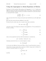
Starting Vortex (2)
Wake shape
of an airfoil
whose angle
of attack was
impulsively
increased to
5 o.
The starting
vortex is
clearly seen

Introduction to Aeroelasticity


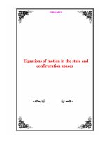
Effect on lift
Initially the angle of
attack is zero. As the

airfoil is symmetrical,
its lift coefficient is also
zero.
c l ( t ) /c l (")
When the change in
angle of attack occurs,
the lift jumps to half its
steady-state value for
the new angle of
attack.
The unsteady lift then
asymptotes towards
its steady-state value
Introduction to Aeroelasticity


Wagner Function (1)
•! The effect of the starting vortex on the
aerodynamic forces around the airfoil can be
modeled by the Wagner function
•! The Wagner function states that the
instantaneous lift at the start of the motion is
equal to half the value of the steady lift (i.e.
the value of the lift if the flow had been
steady)
•! The instantaneous lift then slowly increases
to reach its steady value as time tends to
infinity
Introduction to Aeroelasticity

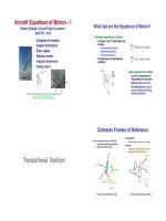
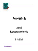
Wagner Function (2)
The Wagner
function is equal to
0.5 when t=0. It
increases
asymptotically to 1.
It can be equally
used to describe an
impulsive change in
angle of attack at
constant airspeed

Introduction to Aeroelasticity


Wagner Function (3)
•! An approximate expression for the Wagner
function is given by
"( t ) = 1# $1e #% 1Ut / b # $2e #% 2Ut / b

•! Where !1=0.165, !2=0.335, !1=0.0455, and
!2=0.3.
•! The lift coefficient variation with time after a
step change in incidence is given by
c l ( t ) = 2"#$( t )

•! So that the lift force variation becomes
l( t ) = "#U 2c$%( t ) = "#Ucw%( t )

Introduction to Aeroelasticity

w=U" is the downwash velocity


Unsteady Motion
•! Unsteady motion can be modeled as a
superposition of many small impulsive
changes in angle of attack
•! The increment in lift due to a small change in
pitch angle at time t0

dw ( t 0 )
dt 0
dl( t ) = "#Uc$( t % t 0 )dw ( t 0 ) = "#Uc$( t % t 0 )
dt 0

•! So that the lift variation at all times can be
obtained by integrating from time -! to time t,
i.e.
t
dw ( t )
l( t ) = "#Uc ' $( t % t 0 )
-&

Introduction to Aeroelasticity

dt 0

0

dt 0


Unsteady Motion (2)

•! Using the thin airfoil theory result
obtained in the first lecture, the
downwash velocity can be written as
$3
&
˙
w ( t ) = U" tot ( t ) = U" ( t ) + h ( t ) + c # x f "˙ ( t )
%4
'

•! For a motion starting at t=0, w=0 for t<0
and w=w(0) at t=0.
•! The lift generated at negative times is
given by
0
dw ( t 0 )
dt 0 = "#Uc$( t )dw (0) = "#Uc$( t ) w (0)
l( t ) t <0 = "#Uc ' $( t % t 0 )
-&
dt
0

Introduction to Aeroelasticity

0


Unsteady Motion (3)
•! Then, the lift at all times is
&
&3
(˙ (
˙
l( t ) = "#Uc *U$ (0) + h (0) + c % x f $ (0)+ ,( t ) +
'4
)
'
)

3
&
&
( ˙˙ (
˙
˙
˙
"#Uc - ,( t % t 0 )*U$ ( t 0 ) + h ( t 0 ) + c % x f $ ( t 0 )+ dt 0
0
'4
)
'
)
t

•! Use integration by parts to get rid of
acceleration terms inside the integral
(these are very difficult to deal with)
•! Result is:
Introduction to Aeroelasticity


Unsteady Motion (4)
&
&3
(˙ (
˙
l( t ) = "#Uc *U$ ( t ) + h ( t ) + c % x f $ ( t )+ ,(0) %
'4
)
'
)

-, ( t % t 0 ) &
&3
(˙ (
˙
"#Uc .
U$ ( t 0 ) + h ( t 0 ) + c % x f $ ( t 0 )+ dt 0
*
0
'4
)
'
)

-t 0
t

•! This equation is the basis of Wagner function
aerodynamics
•! It includes the effect of the entire motion
history of the system in the calculation of the
current lift force
Introduction to Aeroelasticity


Fourier Transform Pair
•! The Wagner Function and Theodorsen’s
Function form a Fourier Transform pair:
t

ik % "( t # t 0 )e ikt 0 dt 0 = C ( k )e ikt
#$

•! Unfortunately, there is a mathematical
difficulty of divergence at -", so the following
is more rigorous:
t

lim ik ' $( t % t 0 )e ikt 0 +"t0 dt 0 = C ( k )e ikt

" #0+

%&

•! Where ! is a small positive number.
Introduction to Aeroelasticity


Fourier Transform Pair (2)
•! In turn, this means that we can derive the Wagner
Function circulatory lift directly from Theodorsen’s
expression, i.e.
&
& 3c
( (
% x f $˙ + =
lc = "#UcC ( k )* U$ + h˙ +
'4
) )
'

&
(
& 3c
(
"#Uc . ,( t % t 0 )* U$˙ ( t 0 ) + h˙˙( t 0 ) +
% x f $˙˙ ( t 0 )+ d/ 0
%'4
)
'
)
t

•! Which becomes more rigorous once the

integration from -" to 0 is carried out:

"
%
" 3c
%
!
lc = !"Uc $U# ( 0 ) + h ( 0 ) + $ ! x f '!! ( 0 ) ' ( (t ) +
#4
&
#
&
"
%
t
" 3c
%
!!
!"Uc ) 0 ( (t ! t0 ) $U!! (t0 ) + h (t0 ) + $ ! x f '!!! (t0 ) 'dt0
#4
&
#
&

Introduction to Aeroelasticity


Moment
•! The aerodynamic moment around the flexural
axis due to the unsteady lift force is simply

mxf(t)=ec l(t)
•! However, for a complete representation of the
aerodynamic force and moment, the added
mass effects must be superimposed, exactly
as was done in the quasi-steady case.
•! The complete equations of motion become
Introduction to Aeroelasticity


Unsteady equations of motion

This type of equation is known as integro-differential since it contains both
integral and differential terms.

Introduction to Aeroelasticity


Integro-differential equations
•! Integro-differential equations cannot be
readily solved in the manner of Ordinary
Differential Equations.
•! A numerical solution can be applied, based
on finite differences, e.g. Houbolt’s Method
•! However, numerical solutions are not very
good for conducting stability analysis
•! The equations must be transformed to ODEs
in order to perform stability analysis
Introduction to Aeroelasticity

Transform to ODEs (1)
•! Use the following substitutions:
The wi variables are
known as the
aerodynamic states. They
arise from the substitution
of the approximate form of
the Wagner function, !, in
the equations of motion.

Introduction to Aeroelasticity


Transform to ODEs (2)
•! The integral in the lift equation can be
expanded by parts. Then, substituting
for the aerodynamic states we obtain

Introduction to Aeroelasticity


Transform to ODEs (3)
•! The integrals have been absorbed by the
aerodynamic states. The full equations of
motion are
M
C

(1)

K

W

Introduction to Aeroelasticity


Transform to ODEs (4)
•! There are two equations with 6
unknowns; 4 more equations are
needed.
•! These can be obtained by noting that
the definitions of wi are of the form
•! Differentiating this equation with time:
Introduction to Aeroelasticity


Leibniz Integral Rule
•! E.g for w1(t):
•! For all wi(t):
(2)

Introduction to Aeroelasticity


Complete Equations
•! Equations (1) and (2) make up the
complete aeroelastic system of equations.
•! Equations (1) are 2nd order Ordinary
Differential Equations (ODEs). They

describe the dynamics of the system
states.
•! Equations (2) are 1st order ODEs. They
describe the dynamics of the aerodynamic
states.
Introduction to Aeroelasticity


Complete Equations (2)
•! Here is the form of the complete equations
•! where

u˙ = Qu

# "M "1 C "M "1 K
%
Q =% I
0
%
W0
$ 0

#1
%
1
%
W0 =
%0
%
$0

Introduction to Aeroelasticity

"M "1 W &
(
0 (,
(
'

# h˙ &
% (
% )˙ (
%h(
% (
)
u =% (
% w1 (
% (
% w2 (
% w3 (
% (
$ w4 '

0 "*1U /b
0
0
0 &
(
0
0 (
0

0
"* 2U /b
1
0
0
"*1U /b
0 (
(
1
0
0
0
"* 2U /b'


Aerodynamic States
•! The aerodynamic states are mathematical
constructs that are used to represent
history effects.
•! As already mentioned several times, the
aerodynamic forces depend not only the
current state of the system but also on the
history of the motion.
•! This history is stored in the aerodynamic
states. After all they are integrals.
Introduction to Aeroelasticity