lab meetings accordion lite 1 PDF 2 27 15 evaluating classifiers in a bag of visual words classification

Does one size really fit all?
Evaluating classifiers in Bag-of-Visual-Words classification
Christian Hentschel, Harald Sack
Hasso Plattner Institute for Software Systems Engineering
Potsdam, Germany

,

ABSTRACT
Bag-of-Visual-Words (BoVW) features that quantize and
count local gradient distributions in images similar to counting words in texts have proven to be powerful image representations. In combination with supervised machine learning approaches, models for various visual concepts can be
learned. While kernel-based Support Vector Machines have
emerged as a de facto standard an extensive comparison of
different supervised machine learning approaches has not
been performed so far. In this paper we compare and discuss the performance of eight different classification models
to be applied in BoVW approaches for image classification:
Na¨ıve Bayes, Logistic Regression, k-nearest neighbors, Random Forests, AdaBoost and linear Support Vector Machines
(SVM) as well as generalized Gaussian kernel SVMs. Our results show that despite kernel-based SVMs performing best
on the official Caltech-101 dataset, ensemble methods fall
only shortly behind. In addition we present an approach for
intuitive heat map-like visualization of the obtained models that help to better understand the reasons of a specific
classification result.

Categories and Subject Descriptors
I.5.4 [Pattern Recognition]: Applications—Computer Vision

General Terms
Algorithms, Experimentation

Keywords
Computer Vision, Bag-of-Visual-Words, Classifier Comparison, Visualization

1.

INTRODUCTION

In this paper, we consider the problem of recognizing the
generic object or scene category of an image. We aim for
automatic classification of an image into one or more classes
Permission to make digital or hard copies of all or part of this work for personal or
classroom use is granted without fee provided that copies are not made or distributed
for profit or commercial advantage and that copies bear this notice and the full citation
on the first page. Copyrights for components of this work owned by others than the
author(s) must be honored. Abstracting with credit is permitted. To copy otherwise, or
republish, to post on servers or to redistribute to lists, requires prior specific permission
and/or a fee. Request permissions from
i-KNOW ’14, September 16 – 19 2014, Graz, Austria
Copyright is held by the owner/author(s). Publication rights licensed to ACM.
ACM 978-1-4503-2769-5/14/09 ...$15.00
/>
describing the depicted content such as car, person or landscape. Within the last decade, Bag-of-Visual-Words (BoVW)
features have been successfully applied in these kind of wholeimage categorization tasks. The approach borrows from
document representation methods in text classification and
compactly summarizes images as 1D histograms of an unordered collection (i.e. bag) of local patch descriptors.
Part of the success of BoVW-based classification systems
results from this generic image description approach. By
simply counting prototypes of image characteristics and discarding any spatial information arbitrary object and scene
categories have been successfully modeled in the past. In
combination with supervised machine learning methods a
category model is trained over the BoVW representation of
a set of training images. As different local image patches

may describe parts of different objects depicted in the same
image the very same representation can be used to model
the car as well as the person that drives the car and the
landscape in the background by providing sufficient training
examples.
In the past, Support Vector Machines (SVM) have emerged
as a de facto standard to learn BoVW-based category models. Especially Radial Basis Function (RBF)-based Kernel
SVMs have been widely applied. While the obtained results are very often satisfactory very few work explicitly targets the comparison of different machine learning methods
for training category models. In this paper we therefore
compare various approaches for image classification based
on BoVW features in terms of the classification accuracy
achieved on the well-known Caltech-101 benchmark dataset1 .
We analyze the performance of eight supervised machine
learning methods for BoVW classification: Na¨ıve Bayes, Logistic Regression, k-nearest neighbors, Random Forests, AdaBoost, linear Support Vector Machines and finally generalized Gaussian kernel SVM (based on standard euclidean and
χ2 distance resp.). Our intention was to evaluate whether
the default choice of Kernel-based Support Vector Machines
is a good choice or whether different classification scenarios
demand for different classification approaches.
This paper is structured as follows: In section 2 we briefly
review the Bag-of-Visual-Words approach for image classification. We describe the relevant steps for BoVW feature
extraction and classification. Section 3 presents the evalu1

The dataset is available at

/>

0.6
0.5
0.4
0.3

0.2
0.1
0.0
0.1
0.2

bet

ter
if
love
fan
whe s
righn
gam t
e
y
hav es
in
gre g
at
ignofuck
ran
shut
fagg t
stupot
i
bitcd
los h
mor er

o
dum n
b
idio
t

of interest are used to represent visual words. By vector
quantization of these features a discrete vocabulary is created. Local features from novel images are assigned to the
closest word in the vocabulary and by counting the number of local features per vocabulary word a BoVW vector is
extracted per image. In [18] the authors give an extensive
overview of the involved steps.

Figure 1: SVM model weights of the 10 most and least
important words in classification of user comments into insults.2

ated classification models in more detail and discusses their
relevance in the context of BoVW classification. In section 4
we present and compare the results obtained on the official
Caltech-101 benchmark dataset. We discuss the individual
performance obtained by each classifier with respect to the
complexity of the classification task and present a novel visualization approach that helps to better understand a learned
category model. Finally, section 5 concludes our paper and
gives a brief outlook on future work.

2.

THE BAG-OF-VISUAL-WORDS MODEL

The Bag-of-Visual-Words (BoVW) approach extends an idea
from text retrieval to visual classification [22]. In text classification systems, each text document is usually represented

by a normalized histogram of word counts. Commonly, this
incorporates all words from a (typically application specific) vocabulary. The vocabulary may exclude certain noninformative words (i.e. stop words) and it usually contains
the words in their stemmed form. A text document is represented by a sparse term vector where each dimension corresponds to a term in the vocabulary and the value of that
dimension is the number of times the term appears in the
document normalized by the total number of vocabulary
words in the document. The term vector is the Bag-ofWords representation – an unsorted collection of vocabulary
words which coined the term bag. In combination with supervised machine learning methods, models for specific text
categories (e.g. Spam mails) can be learned. Typically, a
model captures the meaning of a category by putting higher
weights to important vocabulary words and lower weights
to lesser important terms based on a set of training examples from either category. An example is given in Fig. 1
where a linear Support Vector Machine (SVM) was trained
on a Bag-of-Words model over a document collection of user
comments. The task is to detect when a comment from a
conversation would be considered insulting to another participant in the conversation. As can be seen, the model puts
high weights on the insulting terms and low weights to terms
usually not connotated with insults.
Similarly, an image can be described as a frequency distribution of visual words, independent of their spatial position in
the image plane. While the notion of a word in natural languages is clear, visual words are more difficult to describe.
Typically, local image features extracted at specific regions
2
Adapted from A. Mueller
/>
Feature representation. Similar to words being local features of a text document, local image patches are considered
local features of an image. Different approaches for sampling these features have been presented in literature. The
authors in [16] compared various affine region detectors and
conclude that the Harris-Affine and Maximally Stable Extremal Regions (MSER) detectors performed well under different conditions. Other approaches avoid region of interest
detection and simply sample local image features at dense
grid points. This is mainly due to the fact that low textured
image regions will be ignored by any detector. However,

as shown in [22], the absence of texture must sometimes be
considered as highly discriminative. A comparison of feature
sampling strategies for BoVW vectors has shown that when
using enough samples, dense random sampling exceeds the
performance of interest point operators [17].
Feature descriptors are used to represent the local neighborhood of pixels surrounding a sampling point. Histogram
of gradient based descriptors have been widely adopted in
the field of BoVW models. The most popular descriptor is
the Scale Invariant Feature Transform (SIFT, [14]) which
aggregates 8 gradient orientations at each of 4 × 4 patches
surrounding the sampling point to a 4 ∗ 4 ∗ 8 = 128 dimensional feature vector. A comparison SIFT with other feature
descriptors presented in [15] showed that SIFT-like descriptors tend to outperform the others. While SIFT was initially
devised for intensity images the authors in [24] report that
SIFT extracted on each channel of a color image (i.e. resulting in a 384 dimensional feature vector) improves image
classification results.

Vocabulary generation. Local feature extraction over a
large corpus of training images results in potentially billions
of features with sometimes only minor variations. In order
to obtain a discretized vocabulary that provides some invariance to small changes within the appearance of objects
and to reduce the computational complexity, the number
of descriptors is reduced by vector quantization approaches.
Most BoVW implementations use k-means to cluster the descriptors of a training image set into k vocabulary words (e.g.
[22, 6, 13]). Other approaches that have been successfully
applied use Gaussian Mixtures [20].

BoVW vector generation. Once generated, the derived
cluster centers are used to describe all images in the same
way: By assigning all features descriptors of each image to
the most similar vocabulary vector, a histogram of visual

word vector frequencies is generated per image. Usually this
is achieved by performing a nearest neighbor search within
the vocabulary. Approximate methods have been reported
to improve retrieval time. The obtained frequency distri-


bution is referred to as Bag-of-Visual-Words and represents
the global image descriptor that can be used in subsequent
machine learning steps – analogous to the aforementioned
Bag-of-Words descriptor on text documents. In Figure 2 the
individual steps of the respective BoVW extraction process
are shown.

3.

BOVW CLASSIFICATION

Based on a set of training images a model for a specific visual
category can be trained using the aforementioned BoVW
representation. We consider the task of image categorization
a binary classification problem of separating positive from
negative examples from each category.
Typically, the learning stage optimizes a weight vector that
emphasizes different BoVW vector dimensions (i.e. visual
words) depending on the classification task – very similar
to learning the importance of individual words for a specific text document class. Very early models for BoVWbased image classification have used probabilistic models
such as Na¨ıve Bayes [6], Latent Dirichlet Allocation (LDA)
[9] and probabilistic Latent Semantic Analysis (pLSA) [21]
that have been later replaced by discriminative models such
as AdaBoost [5] and Support Vector Machines (SVM) [23].

While SVMs have become the default choice in most BoVWbased image classification approaches an extensive comparison between different machine learning methods has not yet
been performed. Here, we evaluate the performance of various models in terms of the obtained average precision scores
(area under the precision-recall curve).

3.1

Naïve Bayes

Na¨ıve Bayes classifiers have been successfully applied for a
long time. Most of their popularity comes from the fact
that classification is very fast and training requires a small
amount of samples to estimate the model parameters (for
a more detailed analysis of why Na¨ıve Bayes works well,
see [25]). Despite the simplified assumption of feature independence they have shown good performance in many realworld situations, first of all document classification and email spam filtering.
Consequently, Na¨ıve Bayes classifiers have been among the
first to be used for BoVW classification. The main intuition
behind this model is that each category has a specific distribution over the vocabulary vectors. As an example, a model
that represents the car category may emphasize vocabulary
words which represent the wheels or the car body while the
model of the person category emphasize vocabulary words
for head and torso. Given a collection of training examples,
the classifier learns different distributions for different categories. The distribution of a category y is parametrized
by the vector θy = (θy1 , . . . , θyn ) where n is the number
of terms in the visual vocabulary and θyi is the probability P (xi | y) of term i appearing in a sample belonging to
category y.
Using a smoothed maximum likelihood estimator, θy is optimized:

Nyi + α
θˆyi =
Ny + αn

(1)

where Nyi = x∈T xi is the number of times the vocabulary
term i appears in a sample of category y in the training set
|
T , and Ny = |T
i=1 Nyi is the total count of all vocabulary
terms for category y.
The smoothing parameter α prevents zero probabilities that
may occur due to vocabulary terms not present at all in any
of the training examples.
In [6] a Na¨ıve Bayes classifier is compared to a linear Support Vector Machine classifier and it is shown that the latter
outperforms the former. Similar results have been reported
in [12]. We nevertheless decided to keep Na¨ıve Bayes in our
comparison and use it as a baseline approach.

3.2

Logistic Regression

Logistic regression is used for binary classification problems,
i.e. where the task is to assign a positive yp or negative yn
label to a novel instance. The general assumption behind
logistic regression is that the probability of a category label
yp being assigned to an image represented by its BoVW
vector x can be written as a logistic sigmoid acting on a
linear function of x so that:
p(yp |x) = σ(wT x)

(2)

with p(yn |x) = 1 − p(yp |x). Here σ(·) is the logistic sigmoid
function. The model parameters w are determined using a
maximum likelihood estimator [3]. Logistic Regression is a
very simple classifier and therefore often used as baseline
classifier.

3.3

K Nearest Neighbors

K Nearest Neighbors classification is an example of instancebased learning: instead of attempting to construct an internal model it simply stores instances of the training data (i.e.
the BoVW vectors of all training images). The idea behind
nearest neighbor methods is to retrieve the k training images
closest in distance to a new image and predict the label from
these training examples based on computation of a simple
majority vote. In other words, the category of an image is
set to the category that has the most representatives among
the k nearest training images. The distance metric used can
be any metric measure, however, standard Euclidean distance is the most common choice. The optimal choice of the
value k depends on the classification task and is typically
optimized by grid search and cross validation.
In order to address computational problems for large training sets approximative methods have been proposed. Most
of them are based on variations of binary search trees [2].
Here, we use a KD-tree data structure.

3.4

Random Forests

The Random-Forest algorithm aggregates decisions by weak
classifiers, which in this case are full decision trees [4]. The
algorithm learns a total of n randomized decision trees, each
built from a sample drawn with replacement (i.e., a bootstrap sample) from the training set. Instead of learning these
trees on the complete set of available features, however, a
random subset of these features is selected. Among the features the algorithm iteratively selects the feature that best
splits the training data into positive and negative samples


Figure 2: Steps of BoVW vector extraction with a simplified vocabulary of 6 terms.

(by minimizing the entropy within the training samples).
This process is repeated until either each child node contains only examples of a single class (i.e. is pure) or all features have been considered. The number of decision trees
n is usually optimized via grid search. Classification is performed by evaluating each tree separately. The prediction
of a new sample is based on the majority vote over all trees.

3.5

AdaBoost

label of xi (+1 or −1), αi being the learned weight of the
training sample xi , and b being the learned bias parameter.
The choice of the kernel function K(xi , x) is crucial for good
classification results. In the beginning of BoVW classification most authors restrained to linear Kernels:
Klinear (x, y) = xT y

(4)

Similar to Random Forests, AdaBoost as presented in [10] is

an ensemble learning method that aggregates a sequence of
individual weak learners. Unlike Random Forests, AdaBoost
uses a weighted sample to focus learning on the most difficult
training examples. Additionally, instead of combining classifiers with equal vote (Random Forests use simple majority
vote) AdaBoost uses a weighted vote.

Later, more complex kernel functions have been used to
model non-linear decision boundaries. Typically, these are
variations of generalized forms of RBF kernels:

Arbitrary classifiers can be used as weak classifiers which is
one of the strength of the AdaBoost approach. However, a
sequence of n decision trees with a limited size of depth d is
commonly used. We use cross validation and grid-search to
optimize both, the number of trees as well as their depth.

where d(x, y) can be chosen to be almost any distance function in the BoVW feature space. The standard Gaussian
RBF kernel employs the squared euclidean distance:

3.6

dL2 (x, y) = x − y

Support Vector Machines

As already mentioned, Support Vector Machines represent
by far the most popular classifiers for BoVW (e.g. see [13,
26, 11]). In the presented binary case the decision function
for a test sample x has the following form:

αi yi K(xi , x) − b

g(x) =

1
Kd−RBF (x, y) = exp(− d(x, y))
γ

(3)

i

where K(xi , x) represents the Kernel function value for the
training sample xi and the test sample x, yi being the class

2
2

(5)

(6)

Another distance that has been successfully used is the χ2
distance that is reported to be better suited when comparing
histogram structures like BoVW vectors:

dχ2 (x, y) =
i

(xi − yi )2

|xi | + |yi |

(7)

The authors in [11] evaluate several factors that impact
BoVW image classification using SVMs and compare sev-


eral kernel functions including linear, Histogram Intersection, Gaussian RBF, Laplacian RBF, sub-linear RBF, and
χ2 RBF. On the PASCAL-2005 data set, the best mean
equal error rates occurred for the latter three of the six kernels. The authors subsequently recommend the χ2 RBF and
Laplacian RBF kernels.

Table 1: Experimental results of different classifiers obtained
on BoVW features extracted from the Caltech-101 dataset.
Reported score is mean Average Precision over all categories.
Additionally, hyperparameters optimized via cross validation are reported.

The kernel parameter γ (see eq. 5) is usually optimized by
grid-search and cross validation. However, Zhang et al. [26]
have shown, that in case of the χ2 RBF kernel function setting this value to the mean value of the χ2 distances between
all training images gives comparable results and reduces the
computational effort.
In this paper we present classification results for linear SVM
as well as Gaussian RBF- and χ2 -kernel based SVMs.

4.

EMPIRICAL EVALUATION

In our experiments we have computed BoVW models for
the 101 classes of the Caltech-101 benchmark dataset [8].
We extract SIFT features at equidistantly sampled regions
(every 6 pixels) on each channel of an image in RGB color
space3 . By concatenating these features we obtain a 384dimensional feature vector at each grid point. These features are used to compute the visual vocabulary by running
a k-means clustering with k = 100 on a random subset of
800.000 RGB-SIFT features taken from the training images
set. Finally, BoVW histograms are computed by assigning
each of the extracted RGB-SIFT feature of an image to its
most similar vocabulary word using an approximate nearest
neighbor classifier. BoVW histograms are further L1 normalized in order to account for varying images sizes.
It should be stated that a vocabulary size of k = 100 is most
likely not optimal. In [6] the impact of the vocabulary size
on the overall classification performance is discussed. The
authors state that larger vocabulary sizes perform better,
within the tested range of 100-2500. However, for the sake
of computational efficiency, we limit the vocabulary size to
k = 100. Since evaluation of different classifiers is based
on identical setups, this does not prevent from comparing
relative accuracy scores. However, it should be stated that
absolute classifier accuracy will probably increase with increasing vocabulary sizes.

4.1

Evaluation Dataset

The Caltech-101 dataset [8] was generated by using Google
Image Search to collect images for the 101 categories and
performing a manual post filtering to get rid of irrelevant images. An additional background clutter category with arbitrary images not falling into any of the categories was added
(The keyword things was used to obtain random images, a

total of 467 images were collected). The number of images
per category vary largely – from 31 (inline skate) to 800
(airplanes). The authors denote, that some preprocessing
has been performed: Categories with a predominant vertical structure were rotated to an arbitrary angle. Categories
where two mirror image views were present, were manually
flipped, so all instances are facing the same direction. Finally, all images were scaled to 300 pixels width.
3
We use the OpenCV 2.4.3 SIFT descriptor implementation:
/>
Classifier

Hyperparameters

mAP

Na¨ıve Bayes

α (smoothing parameter)

0,480

k nearest neighbors

k (no. of nearest neighbors)

0,524

Logistic Regression

C (regularization)

0,548

linear SVM

C (regularization)

0,554

RBF kernel SVM

C (regularization), γ (kernel
coefficient)

0,593

Random Forest

n (no. of decision trees)

0,612

AdaBoost

n (no. of decision trees), d
(depth of each decision tree)

0,632

χ2 -kernel SVM

C (regularization)5

0,674

4.2

Experimental Setup

Each category model was trained under identical conditions.
We first have split the set of images of any category (including the background class) into 50% training and 50%
testing data. Subsequently, we have trained models for each
category using the machine learning approaches presented
in Section 3. Each model was trained in a binary setting
taking the training images of the respective class as positive and the training images from the background class as
negative examples. Hyperparameters for each model were
optimized in a 3-fold nested cross validation (if applicable).
We have used implementations for the various algorithms as
provided by the scikit-learn4 machine learning library [19].
Finally, all models were tested on the aforementioned testing data. Results as well as the particular parameters that
were optimized are reported in Table 1.
We compute the Average Precision (AP) for all categories
based on the aforementioned evaluation set using the respective models that have been trained with the hyperparameters that showed best results during cross validation.
Finally, we averaged the AP scores of a classifier over all categories to obtain the mean Average Precision (mAP) score
that is reported in Table 1. The mAP score is used as a single number to evaluate the overall performance of a single
classifier and compare different classifiers.

4.3

Discussion

The mAP scores reported in Table 1 indicate a superior
performance for χ2 -kernel SVMs. These findings are in line
with the results reported by the authors of [11] who recommend χ2 -kernel SVMs for use with BoVW-based models.
Likewise, the comparatively poor performance of the Na¨ıve
Bayes classifier follows prior experimental results. Therefore, Na¨ıve Bayes is recommended to be used for obtaining
baseline results only or whenever strong requirements for
retrieval time need to be met, e.g. for very large datasets.
4

scikit-learn:


Surprisingly, both ensemble methods (Random Forests as
well as AdaBoost) outperform the standard Gaussian RBF
by 2 − 3% which again performs only slightly better (app.
4%) than the linear SVM model and significantly worse (8%)
than the χ2 -based counter part. These findings emphasize
the fact that the decision for the right kernel is crucial to
good classification results. Kernel-based SVMs on the other
hand come with a couple of disadvantages most of all an
increased evaluation time during classification due to the
fact that an possibly complex kernel function needs to be
computed between each support vector and a given testing
example. In these cases, the use of either ensemble method
will reduce classification time with only minor loss in accuracy. Finally, the mAP scores between the worst (Na¨ıve
Bayes) and the best (χ2 -kernel SVM) differ only by 19%
which should be attributed to the fact that the Caltech-101
dataset is a comparatively easy dataset. The covered categories all represent objects (rather than complex scenes)
and most images depict the respective object centered and

at a similar scale. More testing with other, more difficult
datasets is required here.
Figure 3 presents the mean average precision obtained by
the best and the worst performing model computed over
different training set sizes as they occur for the various categories in the Caltech-101 dataset. The scores indicate a
correlation between training set size and the obtained classification accuracy with more training data resulting in higher
performance. This correlation has been asserted in previous
work (e.g. see [1]) and is especially true for high variance
data such as BoVW models. While in general the classification performance based on comparatively few training data
points varies strongly a few outliers featuring considerably
high mAP scores for both classifiers are visible (categories:
minaret, car side and leopards). A closer look into these
categories reveals that all training images taken from the
minaret category have been rotated by an arbitrary angle
(cf. Sec. 4.1), which presumably imposes a strong bias on
both models. A very similar observation can be made for the
category leopards: most images are surrounded by a more
or less prominent black border.

4.4

Model Visualization

By visualizing the learned influence of individual vocabulary
terms similar to the visualization of the most and least important words of the Bag-of-Words model presented in Fig.

1.0

"minaret"

"car side"
"leopards"

0.8

mAP

The performance of the k nearest neighbor classifier performs only slightly better than the Na¨ıve Bayes model. We
assume this is mainly due to the fact of KNN being a low
bias/high variance approach, which easily overfits on most
of the categories due to the small number of training examples. While both models do not achieve competitive performance, their strong advantage is the relatively low training
effort required. Linear SVM and Logistic regression show
similar performance which can be attributed to both computing a very similar linear model. The advantage of a Logistic regression model over Support Vector machines is that
the former provides an intuitive probabilistic interpretation.
Moreover, extensions have been presented that make it easy
to iteratively update a Logistic Regression model by adding
more training images (using online gradient descent methods).

"watch"

0.6
0.4
0.2
0.0
0

NaiveBayes
chi2
50

100

150
200
250
number of training samples

300

350

400

Figure 3: MAP scores of Na¨ıve Bayes and χ2 -kernel SVM
classifiers computed over different training data sizes.

1 we were able to validate our assumption of dataset artifacts (black border and rotation) having a strong impact on
the overall classification outcome. Since each feature of a
BoVW-vector corresponds to a visual word in the vocabulary and the value of each feature is generated by binning
local SIFT descriptors to the most similar visual word we
can extend the learned importance scores (i.e. BoVW feature weights) of a model to the respective SIFT descriptors.
By highlighting the support regions of SIFT descriptors assigned to important visual words using a heat map like representation we are able to visualize the influence each individual pixel has on the overall classification result. Kernelbased SVMs, however, such as the best-performing χ2 -based
solution prevent deducing individual feature weights due to
the implicit mapping into higher dimensional kernel spaces.
AdaBoost on the other hand allows for immediate extraction of features weights as it selects features based on their
capability of solving the classification problem by computing
the decrease in entropy of the obtained class separation. We
use this mean decrease in impurity over all decision trees in
an ensemble as direct indicator for feature importance.
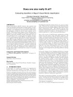
Figure 4 shows examples of heat maps generated for correctly classified test samples of the categories minaret and

leopards. For reasons of clarity we limit the visualized pixel
contributions to the most important visual words, i.e. only
the upper quartile of the importance scores obtained per visual word are shown. Darker areas mark more important
regions and white pixels have least impact on the classification result. Considering Fig. 4b the model has picked
up the textureless black background induced by the rotation of the original picture as highly relevant (hence, the
original intention of the dataset authors to reduce the impact of dominant vertical structures by rotation caused new
artifacts and dominant edges). Similarly, in Fig. 4a the upper end leftermost black border surrounding the picture of
the leopards category has been learned as important characteristic. Since negative training images taken from the
background class possess neither black borders nor rotation
artifacts, these properties are represented by a very specific
distribution over the vocabulary vectors and therefore easily learned even by comparatively simple models such as
Na¨ıve Bayes (χ2 -kernel SVM performs only slighty better
than Na¨ıve Bayes, see Fig. 3). The essential properties of


(a) Category: leopards

(b) Category: minaret

(c) Category: car side

(d) Category: watch

Figure 4: Visualizations of feature importances of the AdaBoost classifier. Top left: original image. Top right: heat map of
the upper quartile of the learned feature importances. Bottom: Desaturated original image with the superposed heat map
(best viewed in color and magnification).

the objects behind each category, however, have not been
learned.
In Fig. 4c and 4d exemplary visualizations of the AdaBoost

models for car side and watch are shown. While the model
for the car category shows many dominant features (e.g.
prominent horizontal lines), features of the category watch
are much less evident as hardly any visual word has been assigned a high importance score. Consequently, the category
is much more difficult to be captured (which may explain
the poor performance of Na¨ıve Bayes when compared to χ2 kernel SVM, see Fig. 3) and requires more sophisticated
approaches to be correctly modeled.

5.

CONCLUSION AND FUTURE WORK

In this paper we have evaluated different classification approaches for BoVW based image classification. Our tests

have shown that Support Vector Machines using χ2 -distance
metric perform best on the Caltech-101 dataset. Moreover, our results indicate that ensemble methods such as
AdaBoost provide a reasonable alternative whenever a kernelbased approach is not practicable, e.g. due to high demands
on computation time. In addition, we have presented an
approach for intuitive verification of a classification model
using a heat-map like representation. Based on this visualization, a closely coupled human and machine analysis enables visual analytics to reveal deficiencies in the trained
models.
Future work will focus on extending our tests to more diverse
datasets. As discussed, the Caltech-101 dataset is very object centric and comparatively easy to learn. We intend to
evaluate the presented classifiers on larger and more complex datasets such as ImageNet [7]. Moreover, we plan to


conduct tests with varying vocabulary sizes as we assume
that the increased sparsity in the BoVW vectors may favor
simpler models such as linear SVMs.

6.

REFERENCES

[1] M. Banko and E. Brill. Scaling to very very large
corpora for natural language disambiguation. In
Proceedings of the 39th Annual Meeting on
Association for Computational Linguistics - ACL ’01,
pages 26–33, Morristown, NJ, USA, 2001. Association
for Computational Linguistics.
[2] J. L. Bentley. Multidimensional binary search trees
used for associative searching, 1975.
[3] C. M. Bishop. Pattern recognition and machine
learning. Springer New York:, 2006.
[4] L. Breiman. Random Forests. Machine Learning,
45:5–32, 2001.
[5] S. Chen, J. Wang, Y. Liu, C. Xu, and H. Lu. Fast
feature selection and training for AdaBoost-based
concept detection with large scale datasets. In
Proceedings of the international conference on
Multimedia - MM ’10, page 1179, New York, New
York, USA, 2010. ACM Press.
[6] G. Csurka, C. R. Dance, L. Fan, J. Willamowski,
C. Bray, and D. Maupertuis. Visual Categorization
with Bags of Keypoints. In Workshop on Statistical
Learning in Computer Vision, ECCV, pages 1–22,
2004.
[7] J. Deng, W. Dong, R. Socher, L.-j. Li, K. Li, and
L. Fei-Fei. ImageNet: A large-scale hierarchical image
database. In 2009 IEEE Conference on Computer

Vision and Pattern Recognition, pages 248–255. IEEE,
June 2009.
[8] L. Fei-Fei, R. Fergus, and P. Perona. Learning
generative visual models from few training examples:
An incremental Bayesian approach tested on 101
object categories. Computer Vision and Image
Understanding, 106(1):59–70, Apr. 2007.
[9] L. Fei-Fei and P. Perona. A Bayesian hierarchical
model for learning natural scene categories. In
Computer Vision and Pattern Recognition, 2005.
CVPR 2005. IEEE Computer Society Conference on,
volume 2, pages 524—-531 vol. 2, 2005.
[10] Y. Freund and R. Schapire. A decision-theoretic
generalization of on-line learning and an application to
boosting. In Computational Learning Theory, volume
904, pages 23–37. 1995.
[11] Y.-G. Jiang, C.-W. Ngo, and J. Yang. Towards
optimal bag-of-features for object categorization and
semantic video retrieval. Proceedings of the 6th ACM
international conference on Image and video retrieval CIVR ’07, pages 494–501, 2007.
[12] F. Jurie and B. Triggs. Creating efficient codebooks
for visual recognition. Tenth IEEE International
Conference on Computer Vision (ICCV’05) Volume 1,
pages 604–610 Vol. 1, 2005.
[13] S. Lazebnik, C. Schmid, and J. Ponce. Beyond Bags of
Features: Spatial Pyramid Matching for Recognizing
Natural Scene Categories. In 2006 IEEE Computer
Society Conference on Computer Vision and Pattern
Recognition - Volume 2 (CVPR’06), pages 2169–2178.
IEEE, 2006.

[14] D. G. Lowe. Distinctive Image Features from
Scale-Invariant Keypoints. International Journal of
Computer Vision, 60(2):91–110, Nov. 2004.
[15] K. Mikolajczyk and C. Schmid. Performance
evaluation of local descriptors. IEEE transactions on
pattern analysis and machine intelligence,
27(10):1615–30, Oct. 2005.
[16] K. Mikolajczyk, T. Tuytelaars, C. Schmid,
A. Zisserman, J. Matas, F. Schaffalitzky, T. Kadir,
and L. V. Gool. A Comparison of Affine Region
Detectors. International Journal of Computer Vision,
65(1-2):43–72, 2005.
[17] E. Nowak, F. Jurie, and B. Triggs. Sampling strategies
for bag-of-features image classification. Computer
˘ SECCV 2006, pages 490–503, 2006.
Visionˆ
aA¸
[18] S. O’Hara and B. Draper. Introduction to the bag of
features paradigm for image classification and
retrieval. arXiv preprint arXiv:1101.3354, (July):1–25,
2011.
[19] F. Pedregosa, G. Varoquaux, A. Gramfort, V. Michel,
B. Thirion, O. Grisel, M. Blondel, P. Prettenhofer,
R. Weiss, V. Dubourg, J. Vanderplas, A. Passos,
D. Cournapeau, M. Brucher, M. Perrot, and
E. Duchesnay. Scikit-learn: Machine Learning in
Python. Journal of Machine Learning Research,
12:2825–2830, 2012.
[20] F. Perronnin and C. Dance. Fisher Kernels on Visual

Vocabularies for Image Categorization. 2007 IEEE
Conference on Computer Vision and Pattern
Recognition, pages 1–8, June 2007.
[21] J. Sivic, B. C. Russell, A. A. Efros, A. Zisserman, and
W. T. Freeman. Discovering objects and their location
in images. In Proceedings of the IEEE International
Conference on Computer Vision, volume I, pages
370–377, 2005.
[22] J. Sivic and A. Zisserman. Video Google: a text
retrieval approach to object matching in videos. In
Proceedings Ninth IEEE International Conference on
Computer Vision, number Iccv, pages 1470–1477.
IEEE, 2003.
[23] C. G. M. Snoek and M. Worring. Concept-Based
ˆ o in
Video Retrieval. Foundations and TrendsA˝
Information Retrieval, 2(4):215–322, 2009.
[24] K. E. A. van de Sande, T. Gevers, and C. G. M.
Snoek. Evaluating color descriptors for object and
scene recognition. IEEE transactions on pattern
analysis and machine intelligence, 32(9):1582–96,
Sept. 2010.
[25] H. Zhang. The Optimality of Naive Bayes. Machine
Learning, 1:3, 2004.
[26] J. Zhang, M. Marszalek, S. Lazebnik, and C. Schmid.
Local Features and Kernels for Classification of
Texture and Object Categories: A Comprehensive
Study. International Journal of Computer Vision,
73(2):213–238, Sept. 2006.