Probability, 2nd edition
Bạn đang xem bản rút gọn của tài liệu. Xem và tải ngay bản đầy đủ của tài liệu tại đây (4.06 MB, 483 trang )
www.it-ebooks.info
www.it-ebooks.info
Probability
www.it-ebooks.info
www.it-ebooks.info
Probability
An Introduction with Statistical
Applications
Second Edition
John J. Kinney
Colorado Springs, CO
www.it-ebooks.info
Copyright © 2015 by John Wiley & Sons, Inc. All rights reserved
Published by John Wiley & Sons, Inc., Hoboken, New Jersey
Published simultaneously in Canada
No part of this publication may be reproduced, stored in a retrieval system, or transmitted in any form or by any
means, electronic, mechanical, photocopying, recording, scanning, or otherwise, except as permitted under
Section 107 or 108 of the 1976 United States Copyright Act, without either the prior written permission of the
Publisher, or authorization through payment of the appropriate per-copy fee to the Copyright Clearance Center,
Inc., 222 Rosewood Drive, Danvers, MA 01923, (978) 750-8400, fax (978) 750-4470, or on the web at
www.copyright.com. Requests to the Publisher for permission should be addressed to the Permissions
Department, John Wiley & Sons, Inc., 111 River Street, Hoboken, NJ 07030, (201) 748-6011, fax (201)
748-6008, or online at />Limit of Liability/Disclaimer of Warranty: While the publisher and author have used their best efforts in
preparing this book, they make no representations or warranties with respect to the accuracy or completeness of
the contents of this book and specifically disclaim any implied warranties of merchantability or fitness for a
particular purpose. No warranty may be created or extended by sales representatives or written sales materials.
The advice and strategies contained herein may not be suitable for your situation. You should consult with a
professional where appropriate. Neither the publisher nor author shall be liable for any loss of profit or any other
commercial damages, including but not limited to special, incidental, consequential, or other damages.
For general information on our other products and services or for technical support, please contact our Customer
Care Department within the United States at (800) 762-2974, outside the United States at (317) 572-3993 or fax
(317) 572-4002.
Wiley also publishes its books in a variety of electronic formats. Some content that appears in print may not be
available in electronic formats. For more information about Wiley products, visit our web site at www.wiley.com.
Library of Congress Cataloging-in-Publication Data:
Kinney, John J.
Probability : an introduction with statistical applications / John Kinney, Colorado Springs,
CO. – Second edition.
pages cm
Includes bibliographical references and index.
ISBN 978-1-118-94708-1 (cloth)
1. Probabilities–Textbooks. 2. Mathematical statistics–Textbooks. I. Title.
QA273.K493 2015
519.2–dc23
2014020218
Printed in the United States of America
10 9 8 7 6 5 4 3 2 1
www.it-ebooks.info
This book is for
Cherry and Kaylyn
www.it-ebooks.info
www.it-ebooks.info
Contents
Preface for the First Edition
xi
Preface for the Second Edition
xv
1. Sample Spaces and Probability
1.1.
1.2.
Discrete Sample Spaces
1
Events; Axioms of Probability
Axioms of Probability
1.3.
1.4.
7
8
Probability Theorems
10
Conditional Probability and Independence
Independence
1.5.
1.6.
1
14
23
Some Examples
28
Reliability of Systems
Series Systems
Parallel Systems
34
34
35
1.7. Counting Techniques
39
Chapter Review
54
Problems for Review
56
Supplementary Exercises for Chapter 1
56
2. Discrete Random Variables and Probability Distributions
2.1.
2.2.
2.3.
Random Variables
61
Distribution Functions
68
Expected Values of Discrete Random Variables
72
Expected Value of a Discrete Random Variable
Variance of a Random Variable
75
Tchebycheff’s Inequality
78
2.4.
2.5.
Binomial Distribution
A Recursion
82
Some Statistical Considerations
88
Hypothesis Testing: Binomial Random Variables
Distribution of A Sample Proportion
98
Geometric and Negative Binomial Distributions
A Recursion
2.10.
72
81
The Mean and Variance of the Binomial
2.6.
2.7.
2.8.
2.9.
61
84
92
102
108
The Hypergeometric Random Variable: Acceptance Sampling
111
Acceptance Sampling
111
The Hypergeometric Random Variable
114
Some Specific Hypergeometric Distributions
116
2.11.
Acceptance Sampling (Continued)
119
vii
www.it-ebooks.info
viii
Contents
Producer’s and Consumer’s Risks
Average Outgoing Quality
122
Double Sampling
124
2.12.
2.13.
121
The Hypergeometric Random Variable: Further Examples
The Poisson Random Variable
130
Mean and Variance of the Poisson
Some Comparisons
132
2.14. The Poisson Process
134
Chapter Review
139
Problems for Review
141
Supplementary Exercises for Chapter 2
128
131
142
3. Continuous Random Variables and Probability Distributions
3.1.
Introduction
146
Mean and Variance
A Word on Words
3.2.
3.3.
150
153
Uniform Distribution
157
Exponential Distribution
159
Mean and Variance
Distribution Function
3.4.
146
Reliability
Hazard Rate
160
161
162
163
3.5. Normal Distribution
166
3.6. Normal Approximation to the Binomial Distribution
3.7. Gamma and Chi-Squared Distributions
178
3.8. Weibull Distribution
184
Chapter Review
186
Problems For Review
189
Supplementary Exercises for Chapter 3
189
175
4. Functions of Random Variables; Generating Functions; Statistical
Applications
4.1.
4.2.
4.3.
Introduction
194
Some Examples of Functions of Random Variables
195
Probability Distributions of Functions of Random Variables
Expectation of a Function of X
4.4.
4.5.
4.6.
4.7.
196
199
Sums of Random Variables I
203
Generating Functions
207
Some Properties of Generating Functions
211
Probability Generating Functions for Some Specific Probability Distributions
Binomial Distribution
213
Poisson’s Trials
214
Geometric Distribution
215
Collecting Premiums in Cereal Boxes
4.8.
4.9.
4.10.
4.11.
4.12.
4.13.
194
Moment Generating Functions
218
Properties of Moment Generating Functions
Sums of Random Variables–II
224
The Central Limit Theorem
229
Weak Law of Large Numbers
233
Sampling Distribution of the Sample Variance
www.it-ebooks.info
216
223
234
213
Contents
4.14.
Hypothesis Tests and Confidence Intervals for a Single Mean
Confidence Intervals, 𝜎 Known
Student’s t Distribution
242
p Values
243
4.15.
Hypothesis Tests on Two Samples
ix
240
241
248
Tests on Two Means
248
Tests on Two Variances
251
4.16. Least Squares Linear Regression
258
266
4.17. Quality Control Chart for X
Chapter Review
271
Problems for Review
275
Supplementary Exercises for Chapter 4
275
5. Bivariate Probability Distributions
5.1.
5.2.
5.3.
5.4.
5.5.
5.6.
283
Introduction
283
Joint and Marginal Distributions
283
Conditional Distributions and Densities
293
Expected Values and the Correlation Coefficient
Conditional Expectations
303
Bivariate Normal Densities
308
Contour Plots
298
310
5.7. Functions of Random Variables
312
Chapter Review
316
Problems for Review
317
Supplementary Exercises for Chapter 5
317
6. Recursions and Markov Chains
6.1.
6.2.
322
Introduction
322
Some Recursions and their Solutions
Solution of the Recursion (6.3)
Mean and Variance
329
6.3.
Random Walk and Ruin
334
Expected Duration of the Game
6.4.
322
326
337
Waiting Times for Patterns in Bernoulli Trials
339
Generating Functions
341
Average Waiting Times
342
Means and Variances by Generating Functions
6.5. Markov Chains
344
Chapter Review
354
Problems for Review
355
Supplementary Exercises for Chapter 6
355
7. Some Challenging Problems
7.1.
7.2.
7.3.
7.4.
7.5.
357
√
My Socks and 𝜋
357
Expected Value
359
Variance
361
Other “Socks” Problems
362
Coupon Collection and Related Problems
Three Prizes
343
363
www.it-ebooks.info
362
x
Contents
Permutations
363
An Alternative Approach
363
Altering the Probabilities
364
A General Result
364
Expectations and Variances
366
Geometric Distribution
366
Variances
367
Waiting for Each of the Integers
367
Conditional Expectations
368
Other Expected Values
369
Waiting for All the Sums on Two Dice
7.6.
7.7.
7.8.
7.9.
7.10.
Conclusion
372
Jackknifed Regression and the Bootstrap
Jackknifed Regression
372
Cook’s Distance
374
The Bootstrap
375
On Waldegrave’s Problem
378
Three Players
7.11.
7.12.
Probabilities of Winning
More than Three Players
378
379
Conclusion
384
On Huygen’s First Problem
384
Changing the Sums for the Players
Decimal Equivalents
Another order
387
Bernoulli’s Sequence
Bibliography
372
378
r + 1 Players
381
Probabilities of Each Player
Expected Length of the Series
Fibonacci Series
383
7.13.
7.14.
7.15.
370
382
383
384
386
387
388
Appendix A. Use of Mathematica in Probability and Statistics
Appendix B. Answers for Odd-Numbered Exercises
Appendix C. Standard Normal Distribution
Index
461
www.it-ebooks.info
453
429
390
Preface for the First Edition
HISTORICAL NOTE
The theory of probability is concerned with events that occur when randomness or chance
influences the result. When the data from a sample survey or the occurrence of extreme
weather patterns are common enough examples of situations where randomness is involved,
we have come to presume that many models of the physical world contain elements of
randomness as well. Scientists now commonly suppose that their models contain random
components as well as deterministic components. Randomness, of course, does not involve
any new physical forces; rather than measuring all the forces involved and thus predicting
the exact outcome of an experiment, we choose to combine all these forces and call the
result random. The study of random events is the subject of this book.
It is impossible to chronicle the first interest in events involving randomness or chance,
but we do know of a correspondence between Blaise Pascal and Pierre de Fermat in the middle of the seventeenth century regarding questions arising in gambling games. Appropriate
mathematical tools for the analysis of such situations were not available at that time, but
interest continued among some mathematicians. For a long time, the subject was connected
only to gambling games and its development was considerably restricted by the situations
arising from such considerations. Mathematical techniques suitable for problems involving randomness have produced a theory applicable to not only gambling situations but also
more practical situations. It has not been until recent years, however, that scientists and
engineers have become increasingly aware of the presence of random factors in their experiments and manufacturing processes and have become interested in measuring or controlling
these factors.
It is the realization that the statistical analysis of experimental data, based on the theory
of probability, is of great importance to experimenters that has brought the theory to the
forefront of applicable mathematics. The history of probability and the statistical analysis
it makes possible illustrate a prime example of seemingly useless mathematical research
that now has an incredibly wide range of practical application. Mathematical models for
experimental situations now commonly involve both deterministic and random terms. It
is perhaps a simplification to say that science, while interested in deterministic models to
explain the physical world, now is interested as well in separating deterministic factors from
random factors and measuring their relative importance.
There are two facts that strike me as most remarkable about the theory of probability.
One is the apparent contradiction that random events are in reality well behaved and that
there are laws of probability. The outcome on one toss of a coin cannot be predicted, but
given 10,000 tosses of the same coin, many events can be predicted with a high degree of
accuracy. The second fact, which the reader will soon perceive, is the pervasiveness of a
probability distribution known as the normal distribution. This distribution, which will be
defined and discussed at some length, arises in situations which at first glance have little in
xi
www.it-ebooks.info
xii
Preface for the First Edition
common: the normal distribution is an essential tool in statistical modeling and is perhaps
the single most important concept in statistical inference.
There are reasons for this, and it is my purpose to explain these in this book.
ABOUT THE TEXT
From the author’s perspective, the characteristics of this text which most clearly differentiate it from others currently available include the following:
• Applications to a variety of scientific fields, including engineering, appear in every
chapter.
• Integration of computer algebra systems such as Mathematica provides insight into
both the structure and results of problems in probability.
• A great variety of problems at varying levels of difficulty provides a desirable
flexibility in assignments.
• Topics in statistics appear throughout the text so that professors can include or omit
these as the nature of their course warrants.
• Some problems are structured and solved using recursions since computers and
computer algebra systems facilitate this.
• Significant and practical topics in quality control and quality production are
introduced.
It has been my purpose to write a book that is readable by students who have some
background in multivariable calculus. Mathematical ideas are often easily understood until
one sees formal definitions that frequently obscure such understanding. Examples allow us
to explore ideas without the burden of language. Therefore, I often begin with examples
and follow with the ideas motivated first by them; this is quite purposeful on my part, since
language often obstructs understanding of otherwise simply perceived notions.
I have attempted to give examples that are interesting and often practical in order to
show the widespread applicability of the subject. I have sometimes sacrificed exact mathematical precision for the sake of readability; readers who seek a more advanced explication
of the subject will have no trouble in finding suitable sources. I have proceeded in the belief
that beginning students want most to know what the subject encompasses and for what it
may be useful. More theoretical courses may then be chosen as time and opportunity allow.
For those interested, the bibliography contains a number of current references.
An author has considerable control over the reader by selecting the material, its order
of presentation, and the explication. I am hopeful that I have executed these duties with due
regard for the reader. While the author may not be described with any sort of precision as
the holder of a tightrope, I have been guided by the admonition: “It’s not healthy for the
tightrope walker to be misunderstood by the person who’s holding the rope.”1
The book makes free use of the now widely available computer algebra systems. I have
used Mathematica, Maple, and Derive for various problems and examples in the book, and
I hope the reader has access to one of these marvelous mathematical aids. These systems
allow us the incredible opportunity to see graphs and surfaces easily, which otherwise would
be very difficult and time-consuming to produce. Computer algebra systems make some
1 Smilla’s
Sense of Snow, by Peter Hoeg (Farrar, Straus and Giroux: New York, 1993).
www.it-ebooks.info
Preface for the First Edition
xiii
parts of mathematics visual and thereby add immensely to our understanding. Derivatives,
integrals, series expansions, numerical computation, and the solution of recursions are used
throughout the book, but the reader will find that only the results are included: in my opinion there is no longer any reason to dwell on calculation of either a numeric or algebraic
sort. We can now concentrate on the meaning of the results without being restrained by the
often mechanical effort in achieving them; hence our concentration is on the structure of
the problem and the insight the solution gives. Graphs are freely drawn and, when appropriate, a geometric view of the problem is given so that the solution and the problem can
be visualized. Numerical approximations are given when exact solutions are not feasible.
The reader without a computer algebra system can still do the problems; the reader with
such a system can reproduce every graph in the book exactly as it appears. I have included
a fairly expensive appendix in which computer commands in Mathematica are given for
many of the examples in which Mathematica was used; this should also ease the translation
to other computer algebra systems. The reader with access to a computer algebra system
should refer to Appendix 1 fairly frequently.
Although I hope the book is readable and as completely explanatory as a probability
text may be, I know that students often do not read the text, but proceed directly to the
problems. There is nothing wrong with this; after all, if the ability to solve practical problems is the goal, then the student who can do this without reading the text is to be admired.
Readers are warned, however, that probability problems are rarely repetitive; the solution
of one problem does not necessarily give even any sort of hint as to the solution of the next
problem. I have included over 840 problems so that a reader who solves the problems can
be reasonably assured that the concepts involving them are understood.
The problem sections begin with the easiest problems and gradually work their way
up to some reasonably difficult problems while remaining within the scope and level of the
book. In discussing a forthcoming examination with my students, I summarize the material
and give some suggestions for practice problems, so I have followed each chapter by a
Chapter Summary, some suggestions for Review Problems, and finally some Supplementary Problems.
FOR THE INSTRUCTOR
Texts on probability often use generating functions and recursions in the solution of many
complex problems; with our use of computer algebra systems, we can determine generating
functions, and often their power series expansions, with ease. The structure of generating
functions is also used to explain limiting behavior in many situations. Many interesting
problems can be best described in terms of recursions; since computer algebra systems
allow us to solve such recursions, some discussion of recursive functions is given. Proofs are
often given using recursions, a novel feature of the book. Occasionally, the more traditional
proofs are given in the exercises.
Although numerous applications of the theory are given in the text and in the problems,
the text by no means exhausts the applications of the theory of probability. In addition to
solving many practical and varied problems, the theory of probability also provides the
basis for the theory of statistical inference and the analysis of data. Statistical analysis is
combined with the theory of probability throughout the book. Hypothesis testing, confidence intervals, acceptance sampling, and control charts are considered at various points in
www.it-ebooks.info
xiv
Preface for the First Edition
the text. The order in which these topics are to be considered is entirely up to the instructor;
the book is quite flexible in allowing sections to be skipped, or delayed, resulting in rearrangement of the material. This book will serve as a first introduction to statistics, but the
reader who intends to apply statistics should also elect a course in applied statistics. In my
opinion, statistics will be the centerpiece of applied mathematics in the twenty-first century.
www.it-ebooks.info
Preface for the Second Edition
I am pleased to offer a second edition of this text. The reasons for writing the book remain
the same and are indicated in the preface for the first edition. While remaining readable and
I hope useful for both the student and the instructor, I want to point out some differences
between the two editions.
• The first edition was written when Mathematica was in its fourth release; it is now
in its ninth release and while its capabilities have grown, some of the commands,
especially those regarding graphs, have changed. Therefore, Appendix 1 is totally
new, reflecting the changes in Mathematica.
• Both first and second editions contain about 120 graphs; these have been mostly
redrawn.
• The problems are of primary importance to the student. Being able to solve them
verifies the student’s mastery of the material. The book now contains over 880
problems, 60 or so of which are new.
• Chapter 7, titled “Some Challenging Problems”, is new. Five problems, or sets
of problems, some of which have been studied by famous mathematicians, are
introduced. Open questions are given, some of which will challenge the reader.
Problems are almost always capable of extension; the reader may do this while
doing a project regarding one of the major problems.
I have profited from comments from both instructors and students who used the first
edition. In a sense I owe a debt to every student of mine at Rose–Hulman Institute of Technology. Heartfelt Thank yous go to Sari Freedman and my editor, Susanne Steitz-Filler
of John Wiley & Sons. Sangeetha Parthasarathy of LaserWords has been very helpful and
patient during the production process. I have been fortunate to rely on the extensive computer skills of my nephew, Scott Carter to whom I owe a big Thank You. But I owe the
greatest debt to my wife, Cherry, who has out up with my long hours in the study. I also
owe a pat on the head for Ginger who allowed me to refresh while guiding me on long
walks through our Old North End neighborhood.
JOHN J. KINNEY
March 4, 2014
Colorado Springs
xv
www.it-ebooks.info
www.it-ebooks.info
Chapter
1
Sample Spaces and Probability
1.1 DISCRETE SAMPLE SPACES
Probability theory deals with situations in which there is an element of randomness or
chance. Some models of the physical world are deterministic, that is, they predict exactly
what will happen under certain circumstances. For example, if an object is dropped from
a height and given no initial velocity, its distance, s, from the starting point is given by
1
s = ⋅ g ⋅ t2 , where g is the acceleration due to gravity and t is the time. If one tried to
2
apply the formula in a practical situation, one would not find very satisfactory results. The
problem is that the formula applies only in a vacuum and ignores the shape of the object
and the resistance of the air as well as other factors. Although some of these factors can be
determined, we generally combine them and say that the result has a random or chance com1
ponent. Our model then becomes s = ⋅ g ⋅ t2 + 𝜖, where 𝜖 denotes the random component
2
of the model. In contrast with the deterministic model, this model is stochastic.
Science often considers stochastic models; in formulating new models, the scientist
may try to determine the contributions of both deterministic and random components of
the model in predicting accurate results.
The mathematical theory of probability arose in consideration of games of chance,
but, as the above-mentioned example shows, it is now widely used in far more practical and
applied situations. We encounter other circumstances frequently in everyday life in which
we presume that some random factors are at work. Here are some simple examples. What
is the chance I will find that all eight traffic lights I pass through on my way to work are
green? What are my chances for winning a lottery? I have a ten-volume encyclopedia that I
have packed in separate boxes. If the boxes become mixed up and I draw the volumes out at
random, what is the chance that my encyclopedia will be in order? My desk lamp has a bulb
that is “guaranteed” to last 5000 hours. It has been used for 3000 hours. What is the chance
that I must replace it before 2000 more hours are used? Each of these situations involves a
random event whose specific outcome is unpredictable in advance.
Probability theory has become important because of the wide variety of practical problems it solves and its role in science. It is also the basis of the statistical analysis of data that
is widely used in industry and in experimentation. Consider some examples. A manufacturer of television sets may know that 1% of the television sets manufactured have defects
of some kind. What is the chance that a shipment of 200 sets a dealer has received contains
2% defective sets? Solving problems such as these has become important to manufacturers who are anxious to produce high quality products, and indeed such considerations play
a central role in what has become known in manufacturing as statistical process control.
Probability: An Introduction with Statistical Applications, Second Edition. John J. Kinney.
© 2015 John Wiley & Sons, Inc. Published 2015 by John Wiley & Sons, Inc.
1
www.it-ebooks.info
2
Chapter 1
Sample Spaces and Probability
Sample surveys, in which only a portion of a population or reference set is investigated,
have become commonplace. A recent survey, for example, showed that two-thirds of welfare recipients in the United States were not old enough to vote. But surely we do not know
that exactly two-thirds of all welfare recipients were not old enough to vote; there is some
uncertainty, largely dependent on the size of the sample investigated as well as the manner in which the survey was conducted, connected with this result. How is this uncertainty
calculated?
As a final example, consider a scientific investigation into say the relationship between
temperature, a catalyst, and pressure in creating a chemical compound. A scientist can
only carry out a few experiments in which several combinations of temperatures, amount
of catalyst, and level of pressure are investigated. Furthermore, there is an element of
randomness (largely due to other, unmeasured, factors) that influence the amount of compound produced. How is the scientist to determine which combination of factors maximizes
the amount of chemical compound? We will encounter many of these examples in this
book.
In some situations, we could measure all the forces involved and predict the outcome
precisely but very often choose not to do so. In the traffic light example, we could, by
knowledge of the timing of the lights, my speed, and the traffic pattern, predict precisely
the color of each light as I approach it. While this is possible, it is probably not worth the
effort, so we combine all the forces involved and call the result “chance.” So “chance” as
we use it does not imply any new or unknown physical forces; it is simply an umbrella
under which we put forces we choose not to measure.
How do we then measure the probability of events such as those described earlier? How
do we determine how likely such events are? Such probability problems may be puzzling
to us since we lack a framework in which to solve them. We lack a strategy for dealing with
the randomness involved in these situations. A sensible way to begin is to consider all the
possibilities that could occur. Such a list, or set, is called a sample space.
We begin here with some situations that are admittedly much simpler than some of
those described earlier; more complex problems will also be encountered in this book.
We will consider situations that we call experiments. These are situations that can be
repeated under identical circumstances. Those of interest to us will involve some randomness so that the outcomes cannot be precisely predicted in advance. As examples, consider
the following:
•
Two people are chosen at random from a group of five people.
•
Choose one of two brands of breakfast cereal at random.
•
Throw two fair dice.
•
Take an actuarial examination until it is passed for the first time.
•
Any laboratory experiment.
Clearly, the first four of these experiments involve random factors. Laboratory experiments involve random factors as well and we would probably choose not to measure all the
factors so as to be able to predict the exact outcome in advance.
Once the conditions for the experiment are set, and we are assured that these
conditions can be repeated exactly, we can form the sample space, which we define as
follows:
Definition
ment.
A sample space is a set of all the possible outcomes from an experi-
www.it-ebooks.info
1.1 Discrete Sample Spaces
3
Example 1.1.1
The sample spaces for the first four experiments mentioned above are as follows:
(a) (Choose two people at random from a group of five people.) Denoting the five
people as A, B, C, D, and E, we find, if we disregard the order in which the persons
are chosen, that there are ten possible samples of two people:
S = {AB, AC, AD, AE, BC, BD, BE, CD, CE, DE}.
This set, S, then comprises the sample space for the experiment.
If we consider the choice of people as random, we might expect that each of
these ten samples occurs about 10% of the time. Further, we see that any particular
person, say B, occurs in exactly four of the samples, so we say the probability that
4
2
= . The reader may be interested
any particular person is in the sample is
10
5
to show that if three people were selected from a group of five people, then the
3
probability a particular person is in the sample is . Here, there is a pattern that we
5
can establish with some results to be developed later in this chapter.
(b) (Choose one of two brands of breakfast cereal at random.) Denote the brands as K
and P. We take the sample space as
S = {K, P},
where the set S contains each of the elementary outcomes, K and P.
(c) (Toss two fair dice.) In contrast with the first two examples, we might consider
several different sample spaces. Suppose first that we distinguish the two dice by
color, say one is red and the other is green. Then we could write the result of a toss
as an ordered pair indicating the outcome on each die, giving say the result on the
red die first and the result on the green die second. Let a sample space be
S1 = {(1, 1), (1, 2), ..., (1, 6), (2, 1), (2, 2), ..., (2, 6), ..., (6, 6)}.
It is useful to see this sample space as a geometric space as in Figure 1.1.
Note that the 36 dots represent the only possible outcomes from the experiment. The sample space is not continuous in any sense in this case and may differ
from our notions of a geometric space.
We could also describe all the possible outcomes from the experiment by
the set
S2 = {2, 3, 4, 5, 6, 7, 8, 9, 10, 11, 12}
since one of these sums must occur when the two dice are thrown.
First die
Second die
6
5
4
3
2
1
.
.
.
.
.
.
1
.
.
.
.
.
.
2
.
.
.
.
.
.
3
.
.
.
.
.
.
4
.
.
.
.
.
.
5
.
.
.
.
.
.
6
Figure 1.1 Sample space for tossing two dice.
www.it-ebooks.info
4
Chapter 1
Sample Spaces and Probability
Which sample space should be chosen? Note that each point in S2 represents
at least one point in S1 . So, while we might consider each of the 36 points in
S1 to occur with equal frequency if we threw the dice a large number of times,
we would not consider that to be true if we chose sample space S2 . A sum of
7, for example, occurs on 6 of the points in S1 while a sum of 2 occurs at only
one point in S1 . The choice of sample space is largely dependent on what sort
of outcomes are of interest when the experiment is performed. It is not uncommon for an experiment to admit more than one sample space. We generally select
the sample space most convenient for the analysis of the probabilities involved in
the problem.
We continue now with further examples of experiments involving randomness.
(d) (Take an actuarial examination until it is passed for the first time.) Letting P and F
denote passing and failing the examination, respectively, we note that the sample
space here is infinite:
S = {P, FP, FFP, FFFP, … }.
However, S here is a countably infinite sample space since its elements can be
counted in the sense that they can be placed in a one-to-one correspondence with
the set of natural numbers {1, 2, 3, 4, … } as follows:
P↔1
FP ↔ 2
FFP ↔ 3
⋅
⋅
⋅
The rule for the one-to-one correspondence is as follows: given an entry in the left
column, the corresponding entry in the right column is the number of the attempt
on which the examination is passed; given an entry in the right column, say n,
consider n − 1F’s followed by P to construct the corresponding entry in the left
column. Hence, the correspondence with the set of natural numbers is one-to-one.
Such sets are called countable or denumerable. We will consider countably infinite
sets in much the same way that we will consider finite sets. In the next chapter, we
will encounter infinite sets that are not countable.
(e) Sample spaces for laboratory experiments are usually difficult to enumerate and
may involve a combination of finite and infinite factors.
Example 1.1.2
As a more difficult example, consider observing single births in a hospital until two girls
are born in a row.
The sample space now is a bit more challenging to write down than the sample spaces
for the situations considered in Example 1.1.1.
www.it-ebooks.info
1.1 Discrete Sample Spaces
5
For convenience, we write the points, showing the births in order and grouped by the
total number of births.
Number of
Births
Sample
Points
Number of
Sample Points
2
GG
1
3
BGG
1
4
BBGG
2
GBGG
5
BBBGG
BGBGG
GBBGG
4
6
BBBBGG
BBGBGG
BGBBGG
GBBBGG
GBGBGG
6
and so on. We note that the number of sample points as we have grouped them follows the
sequence 1, 1, 2, 4, 6, … , which we recognize as the beginning of the Fibonacci sequence.
The Fibonacci sequence is found by starting with the sequence 1, 1. Subsequent entries are
found by adding the two immediately preceding entries. However, we only have evidence
that the Fibonacci sequence applies to a few of the groups of points in the sample space.
We will have to establish the general pattern in this example before concluding that the
Fibonacci sequence does indeed give the number of sample points in the sample space. The
reader may wish to do that before reading the following paragraphs!
Here is the reason the Fibonacci sequence occurs: consider a sequence of B’s and G’s
in which GG occurs for the first time at the nth birth. Let an denote the number of ways
in which this can occur. If GG occurs for the first time on the nth birth, there are two
possibilities for the beginning of the sequence. These possibilities are mutually exclusive,
that is, they cannot occur together.
One possibility is that the sequence begins with a B and is followed for the first time
by the occurrence of GG in n − 1 births. Since we are requiring the sequence GG to occur
for the first time at the n − 1st birth, this can occur in an−1 ways.
The other possibility for the beginning of the sequence is that the sequence begins
with G, which must then be followed by B (else the pattern GG will occur in two births)
and then the pattern GG occurs in n − 2 births. This can occur in an−2 ways. Since the
sequence begins either with B or G, it follows that
an = an−1 + an−2 , n ≥ 4,
where a2 = a3 = 1,
(1.1)
which describes the Fibonacci sequence.
The sequences for which GG occurs for the first time in 7 births can then be found
by writing B followed by the sequences for 6 births and by writing GB followed by GG in
5 births:
www.it-ebooks.info
6
Chapter 1
Sample Spaces and Probability
B|BBBBGG
B|BBGBGG
B|BGBBGG
B|GBBBGG
B|GBGBGG
GB|BBBGG
GB|BGBGG
GB|GBBGG
Formulas such as ((1.1)) often describe a problem in a very succinct manner; they are
called recursions because they describe one value of a function, here an , in terms of other
values of the same function; in addition, they are easily programmed. Computer algebra
systems are especially helpful in giving large number of terms determined by recursions.
One can find, for example, that there are 46,368 ways for the sequence GG to occur for the
first time on the 25th birth. It is difficult to imagine determining this number without the
use of a computer.
EXERCISES 1.1
1. Show the sample space when 3 people are selected from a group of 5 people. Verify
the fact that any particular person in the selected group is 3/5.
2. In Example 1.1.2, show all the sample points where the births of two girls in a row
occur in 8 or 9 births.
3. An experiment consists of drawing two numbered balls from a box of balls numbered
from 1 to 9. Describe the sample space if
(a) the first ball is not replaced before the second is drawn.
(b) the first ball is replaced before the second is drawn.
4. In the diagram below, A, B, and C are switches that may be closed (current flows
through the switch) or open (current cannot flow through the switch). Show the sample
space indicating all the possible positions of the switches in the circuit.
A
B
C
www.it-ebooks.info
1.2 Events; Axioms of Probability
7
5. Items being produced on an assembly line can be good (G) or not meeting specifications
(N). Show the sample space for the next five items produced by the assembly line.
6. A student decides to take an actuarial examination until it is passed, but will attempt
the test at most five times. Show the sample space.
7. In the World Series, games are played until one of the teams has won four games. Show
all the points in the sample space in which the American League (A) wins the series
over the National League (N) in at most six games.
8. We are interested in the sequence of male and female births in five-child families. Show
the sample space.
9. Twelve chips numbered 1 through 12 are mixed in a bowl. Two chips are drawn successively and without replacement. Show the sample space for the experiment.
10. An assembly line is observed until items of both types—good (G) items and items not
meeting specification (N)—are observed. Show the sample space.
11. Two numbers are chosen without replacement from the set {2, 3, 4, 5, 6, 7}, with the
additional restriction that the second number chosen must be smaller than the first.
Describe an appropriate sample space for the experiment.
12. Computer chips coming off an assembly line are marked defective (D) or nondefective
(N). The chips are tested and their condition listed. This is continued until two consecutive defectives are produced or until four chips have been tested, whichever occurs
first. Show a sample space for the experiment.
13. A coin is tossed five times and a running count of the heads and tails is kept (so the
number of heads and the number of tails tossed so far is recorded at each toss). Show
all the sample points where the heads count always exceeds the tails count.
14. A sample space consists of all the linear arrangements of the integers 1, 2, 3, 4, and 5.
(These linear arrangements are called permutations).
(a) Use your computer algebra system to list all the sample points.
(b) If the sample points are equally likely, what is the probability that the number 3 is
in the third position?
(c) What is the probability that none of the integers occupies its natural position?
1.2 EVENTS; AXIOMS OF PROBABILITY
After establishing a sample space, we are often interested in particular points, or sets of
points, in that sample space. Consider the following examples:
(a) An item is selected at random from a production line. We are interested in the
selection of a good item.
(b) Two dice are tossed. We are interested in the occurrence of a sum of 5.
(c) Births are observed until a girl is born. We are interested in this occurring in an
even number of births.
Let us begin by defining an event.
Definition
An event is a subset of a sample space.
Events then contain one or more elementary outcomes in the sample space.
www.it-ebooks.info