Incorporating bioclimatic and biogeographic data in the construction of plant distribution 2014
Bạn đang xem bản rút gọn của tài liệu. Xem và tải ngay bản đầy đủ của tài liệu tại đây (791.77 KB, 16 trang )
This article was downloaded by: [Universidad de Leon]
On: 02 December 2014, At: 07:19
Publisher: Taylor & Francis
Informa Ltd Registered in England and Wales Registered Number: 1072954 Registered office: Mortimer House,
37-41 Mortimer Street, London W1T 3JH, UK
Plant Biosystems - An International Journal Dealing
with all Aspects of Plant Biology: Official Journal of the
Societa Botanica Italiana
Publication details, including instructions for authors and subscription information:
/>
Incorporating bioclimatic and biogeographic data in the
construction of species distribution models in order to
prioritize searches for new populations of threatened
flora
a
a
ab
ab
a
E. Alfaro-Saiz , M.E. García-González , S. del Río , Á. Penas , A. Rodríguez & R. Alonsoa
Redondo
a
Department of Biodiversity and Environmental Management, University of León, Spain
b
Mountain Livestock Institute, CSIC-University of León, Spain
Accepted author version posted online: 13 Oct 2014.Published online: 25 Nov 2014.
To cite this article: E. Alfaro-Saiz, M.E. García-González, S. del Río, Á. Penas, A. Rodríguez & R. Alonso-Redondo (2014):
Incorporating bioclimatic and biogeographic data in the construction of species distribution models in order to prioritize
searches for new populations of threatened flora, Plant Biosystems - An International Journal Dealing with all Aspects of
Plant Biology: Official Journal of the Societa Botanica Italiana, DOI: 10.1080/11263504.2014.976289
To link to this article: />
PLEASE SCROLL DOWN FOR ARTICLE
Taylor & Francis makes every effort to ensure the accuracy of all the information (the “Content”) contained
in the publications on our platform. However, Taylor & Francis, our agents, and our licensors make no
representations or warranties whatsoever as to the accuracy, completeness, or suitability for any purpose of the
Content. Any opinions and views expressed in this publication are the opinions and views of the authors, and
are not the views of or endorsed by Taylor & Francis. The accuracy of the Content should not be relied upon and
should be independently verified with primary sources of information. Taylor and Francis shall not be liable for
any losses, actions, claims, proceedings, demands, costs, expenses, damages, and other liabilities whatsoever
or howsoever caused arising directly or indirectly in connection with, in relation to or arising out of the use of
the Content.
This article may be used for research, teaching, and private study purposes. Any substantial or systematic
reproduction, redistribution, reselling, loan, sub-licensing, systematic supply, or distribution in any
form to anyone is expressly forbidden. Terms & Conditions of access and use can be found at http://
www.tandfonline.com/page/terms-and-conditions
Plant Biosystems, 2014
/>
ORIGINAL ARTICLE
Incorporating bioclimatic and biogeographic data in the construction of
species distribution models in order to prioritize searches for new
populations of threatened flora
´ LEZ1, S. DEL RI´O1,2, A
´ . PENAS1,2, A. RODRI´GUEZ1,
E. ALFARO-SAIZ1, M.E. GARCI´A-GONZA
1
& R. ALONSO-REDONDO
Downloaded by [Universidad de Leon] at 07:19 02 December 2014
1
Department of Biodiversity and Environmental Management, University of Leo´n, Spain and 2Mountain Livestock Institute,
CSIC-University of Leo´n, Spain
Abstract
The aim of this study was to analyse the usefulness of incorporating bioclimatic and biogeographic data into digital species
prediction and modelling tools in order to identify potential habitats of rare or endangered flora taxa. Species distribution
models (SDMs) were obtained using the Maximum entropy algorithm. Habitat suitability maps were based on sites of known
occurrence of studied species. The study showed that highly reliable habitat prediction models can be obtained through the
inclusion of bioclimatic and biogeographic maps when modelling these species. The resultant SDMs are able to fit the search
area more closely to the characteristics of the species, excluding the percentage of highly suitable areas that are located far
from the known distribution of the taxon, where the probability of finding the plant is low. Therefore, it is possible to
overcome one of the most commonly encountered problems in the construction of rare or threatened flora taxa SDMs,
derived from the low number of initial citations. The resulting SDMs and the vegetation map enable prioritization of the
search for new populations and optimization of the economic and human resources used in the collection of field data.
Keywords: Bioclimatology, biogeography, Maxent, rare species, SDMs, threatened flora
Introduction
Species distribution models (SDMs) based on
known occurrence conditions at study sites constitute an important analytical tool which incorporates
the use of Geographic Information Systems (GIS)
and remote sensing tools for conservation biology
studies (Peterson 2001). In recent years, SDMs have
been used successfully in conservation studies on
various threatened taxa and have proved valuable in
research aimed at locating new populations of rare
species (Bourg et al. 2005; Guisan et al. 2006;
Williams et al. 2009), predicting the habitat of
endemic species (Moreno et al. 2011), prioritizing
areas for the reintroduction of threatened species
(Martı´nez-Meyer et al. 2006; Adhikari et al. 2012),
predicting future situations under several climatechange scenarios (De´samore´ et al. 2012; Da´vila et al.
2013) and in studies involving biogeography (Lobo
et al. 2001; Luoto et al. 2006). Earlier research into
the modelling of threatened flora in Spain focussed
on other species and used different methods (Benito
et al. 2009; Felicı´simo 2011).
Applied specifically to rare species, for which data
are often poor, traditional sampling methods are
limited because many of the randomly-selected sites
are unlikely to contain the species studied (Guisan
et al. 2006). SDMs therefore constitute an accurate
tool that allows the stratified sampling of new
populations and generate a more efficient automated
identification of priority search areas. However,
habitat modelling of these rare or threatened taxa
poses several challenges. These plants tend to have
restricted distribution ranges and limited dispersal
ability. Moreover, the number of samples is often
very small if the taxa have a restricted distribution or
are locally endemic, which gives rise to problems
when working with few known occurrence records,
since values lower than 15 – 20 occurrences can
artificially increase the consistency of the model
Correspondence: E. Alfaro-Saiz, Department of Biodiversity and Environmental Management, Faculty of Environmental and Biological Sciences, University of
Leo´n, Vegazana Campus, 24071 Leo´n, Spain. Tel: þ34 987291554. Fax: þ34 987291563. Email:
q 2014 Societa` Botanica Italiana
Downloaded by [Universidad de Leon] at 07:19 02 December 2014
2
E. Alfaro-Saiz et al.
Figure 1. Location of the studied area and distribution map of the studied taxa on a 10 km £ 10 km grid in Castilla y Leo´n (Spain).
(Veloz 2009). Furthermore, some of these species
have very strict ecological requirements that are
difficult to capture in maps of the resolution normally
used in models of this kind, and the resulting maps
fail to take into account the dispersal capacity of
different species, which in some areas may be very
low due to topography and relief (Mateo et al. 2011).
Consequently, suitability maps of rare or threatened
taxa often identify areas as suitable when they are far
from the actual distribution of the species and where,
although the potential habitat may be very large, the
actual probability of finding the studied species is
very low.
The findings reported here show that some of the
errors often occurring when calculating potential
habitats can be solved by incorporating bioclimatic
and biogeographic data (thermotype, ombrotype and
biogeographical sectors) into the model. Since
bioclimatology studies the relationship between
climate, plant distribution and plant communities
(Rivas-Martı´nez et al. 2011), this approach would
currently appear to be the most useful. Plants and
plant communities act as bioindicators for marking
out different bioclimatological and biogeographic
units.
Much more realistic SDMs are obtained using a
taxon-distribution approach. These models can
predict new locations while significantly reducing
the search area in remote areas of known distribution. The overall aim was to design tools that will
help to find new populations of rare or endangered
taxa, this being crucial for their conservation.
Materials and methods
The taxa
To calibrate the SDMs required for this study, five
protected taxa included in the Decree on Protected
Flora of Castilla y Leo´n (JCYL 2007) were modelled.
The taxa studied included three regional endemics
with a very small number of populations (Draba
hispanica subsp. lebrunii (P. Monts.) Laı´nz, Echium
cantabricum (Laı´nz) Fern. Casas & Laı´nz and
Petrocoptis pyrenaica subsp. viscosa (Rothm.)
P. Monts. & Fern. Casas), a widely distributed
regional endemic (Fritillaria legionensis Llamas &
Andre´s) and a taxon with Eurasian distribution but
very rare at regional level (Lathraea squamaria L.).
Taxa with heterogeneous distribution ranges and
abundance, and different ecological requirements,
were selected, with a view to enabling an objective
evaluation of the proposed method in a range of
possible scenarios.
Figure 1 shows the location of the study area and
distribution of the taxa on a 10 km £ 10 km grid in
Castilla y Leo´n (Spain). Information about the taxa
Downloaded by [Universidad de Leon] at 07:19 02 December 2014
Bioclimatic –biogeographic data in SDMs
studied and their conservation status is provided in
online Appendix I.
An exhaustive bibliographic review was performed
in order to create distribution maps for these taxa in
Castilla y Leo´n. Existing bibliographic locations,
herbarium sheets of LEB-Jaime Andre´s Rodrı´guez
and locations from Vascular Flora of Castilla y Leo´n
Database (JCYL 2002–2012) were used. Moreover,
authors’ field notes, geographically located by means of
Garmin Global Positioning System (GPS) technology
(capture error: 1–10 m), were incorporated. Every
point obtained from these various sources was tested in
the field and georeferenced in order to draw up
occurrence point maps. Forty-three occurrence points
were used to construct the SDMs for D. hispanica
subsp. lebrunii, 5 points for E. cantabricum, 17 points for
F. legionensis, 9 points for L. squamaria and 13 points for
P. pyrenaica subsp. viscosa.
The variables
This study used a combination of variables traditionally
used in SDM research (Guisan et al. 2006; Williams
et al. 2009), together with qualitative bioclimatic and
biogeographic variables. Predictor layers were
resampled at 100 m resolution (when required),
because Maximum entropy (Maxent) algorithm confirmed its strengths also at fine resolutions when
modelling endemic species (van Gils et al. 2012).
A correlation analysis (Pearson coefficient) was carried
out using the SPSS software package (SPSS 2010).
No variable was removed because the correlation
coefficient was less than 0.75 (Rissler & Apodaca 2007).
Categorical variables. Biogeographic variables: In
order to include biogeography as a predictor variable
in the models, the biogeographical map of Spain and
Portugal drawn up by Rivas-Martı´nez et al. (2002)
was used. The nomenclature follows Rivas-Martı´nez
et al. (2011). The biogeography variable was
transformed into a raster map. Sector level was
considered appropriate for the purpose, because it
represents an area containing distinctive taxa and
plant communities, some of which are endemic,
endowing the space with a geographical unity and
enabling it to be differentiated from other nearby
areas (Rivas-Martı´nez 2007). Detailed vegetation
maps clearly circumscribe the potential habitats for
each species, but may lose information when
transformed into raster format at the same resolution
as the other variables in order to incorporate them
into modelling software (Mateo et al. 2011).
Qualitative bioclimatic variables: Thermotype and
ombrotype bioclimatic maps of Castilla y Leo´n (del
Rı´o 2005) were used. The thermotype map was
created using the compensated thermicity index (Itc,
if the value of Itc , 120, or the value of Ic $ 21) and
3
positive temperature (Tp) as reference indices
(Rivas-Martı´nez et al. 2011) (online Appendix II).
This map establishes isoregions using Itc or Tp value
ranges, i.e. areas that reflect the severity of the cold,
a limiting factor for many species and plant
communities. The ombrotype map was created
using the annual ombrothermic index (Io) (RivasMartı´nez et al. 2011) as the reference bioclimatic
index (online Appendix II). This map establishes
isoregions using Io values, i.e. areas that reflect
overall water availability, distinguishing between
large vegetation structures. Maps were created
using the altitude difference between two thermopluviometric stations and their corresponding Io
and Itc values. These data were used to calculate the
altitude levels at which thermotype and ombrotype
change (del Rı´o 2005).
The qualitative bioclimatic variables were transformed into a raster map.
Lithologic variables: The lithologic information
provided by the geological survey map of Castilla y Leo´n
(JCYL 1997) was used. The lithological map available
in vector format was transformed into raster maps.
Numerical variables. Quantitative bioclimatic and
climatic variables: Maps representing climatic parameters were obtained from the Climatic Digital
Atlas of the Iberian Peninsula (Ninyerola et al. 2005)
at 200 m spatial resolution. These maps were
transformed to obtain the following variables (online
Appendix II): continentality index (Ic), thermicity
index (It), summer precipitation (Ps), summer
temperature (Ts) (Rivas-Martı´nez et al. 2011),
degree-days (GDD) from June to September
(Arnold 1960) and Thornthwaite’s monthly potential evapotranspiration index (PE), calculated for the
month of August (Thornthwaite 1948).
Topographic variables: Topographic variables were
obtained from the digital elevation model (DEM) of
Castilla y Leo´n with a resolution of 100 m, available
online (). In addition to the altitude
map, aspect, slope and solar radiation maps were
obtained from the DEM.
Modelling procedures
To model the geographical distribution of species,
Maxent 3.3.3k was used. This software enables
estimation of the geographic distribution of the
suitable habitat of taxa for a set of pixels in the study
region based on Maxent, and represents a mathematical algorithm whose predictions and inferences
can be made from incomplete information (Phillips
et al. 2006; Phillips & Dudı´k 2008; Elith et al. 2011).
There were several reasons for using the Maxent
algorithm. Maxent is a general-purpose machine
method with a simple and precise mathematical
4
E. Alfaro-Saiz et al.
Table I. Results obtained for the two groups of models.
Downloaded by [Universidad de Leon] at 07:19 02 December 2014
Draba
Suitable (%)
Very suitable (%)
Total suitable (%)
AUC
Sensitivity
Specificity
Altitude
Aspect
Biogeography
GDD
PE in August
Ic
It
Lithology
Ombrotype
Slope
Solar radiation
Ps
Ts
Thermotype
Echium
Fritillaria
Lathraea
Petrocoptis
Model 1
Model 2
Model 1
Model 2
Model 1
Model 2
Model 1
Model 2
Model 1
Model 2
0.05
0.02
0.07
0.998
1
0.999
0.1
1.1
7.3
0.9
0.1
5.1
0.2
28.4
2.8
0.1
0
0
0
53.9
0.11
0.04
0.15
0.998
1
0.998
1.6
1.2
0.11
0.02
0.13
1
0.8
0.998
0
0.1
36.5
2.9
0
1.3
0.1
36.8
0.2
0
3
0.9
6.5
11.7
0.10
0.04
0.14
0.999
0.8
0.998
2.52
0.35
2.87
0.992
1
0.97
0.9
3
18.2
15.8
0.9
0.7
2.6
16.9
19.4
1.8
1.8
2.6
5.1
10.3
4.02
0.52
4.54
0.991
1
0.95
0.4
4.2
4.28
0.67
4.95
0.983
1
0.95
0
1.1
22.7
0
3.2
0
0.5
24.7
16.1
0
0.7
6.4
0.8
23.8
7.13
1.67
8.80
0.983
1
0.91
0
0.6
0.09
0.05
0.14
0.999
1
0.999
0
3.6
31.5
0
0
0.8
0
37.2
1.6
3.3
3.9
1.3
0
16.7
0.36
0.18
0.54
0.999
1
0.994
0.5
3.3
22.1
0.2
9.3
1.6
63.8
0.1
0.1
0.1
0
0.1
1.8
0
0.6
0.5
45.7
0.4
5.5
0
45.3
58.2
0.9
0.4
7.6
17.7
2.9
0.8
3.9
3
0
12.9
0.2
0
59.6
0.2
1.5
22.9
2.1
0
0
1.6
0
64.9
15.2
14.2
0.2
0
Notes: The first two rows show the percentages obtained from modelling for each habitat suitability category. The third row shows the
percentage of total habitat considered suitable. AUC represents the value obtained for this parameter using the Maxent software. The other
rows show the relative contributions of the environmental variables to the model.
formulation; it allows the use of qualitative variables
and it boasts a number of features that render it well
suited for species distribution modelling (Phillips
et al. 2006). Furthermore, it compares favourably
with other modelling methods, especially when
working with small sample sizes, making it suitable
for modelling rare or endangered species, as shown in
several studies (Elith et al. 2006; Hernandez et al.
2006; Phillips et al. 2006; Pearson et al. 2007;
Williams et al. 2009; Mateo et al. 2010; Moreno et al.
2011; Babar et al. 2012).
The default values taken by the software for the
proper convergence of the algorithm were 500 as the
maximum number of iterations to 0.00001 as the
convergence limit. The model was run 10 times using
bootstrapped subsamples, 5 times for E. cantabricum
and 9 times for L. squamaria, corresponding to the
presence points’ numbers. Model results were averaged
across the bootstrap replicates. The final maps were
made using the “logistic” output mode, which is more
readily interpretable (Phillips 2008), and accessed in
ASCII format.
Information relating to the occurrence points of
the taxa studied was combined with the following
variables: biogeographic (sector level), qualitative
bioclimatic (ombrotype and thermotype), quantitative bioclimatic and climatic (Ic, It, Ps, Ts, GDD and
PE), topographic (slope, solar radiation, altitude and
aspect) and lithologic.
To perform the final calculations and compare
models, these were simplified, by reducing them to
three habitat suitability classes (absence, suitable and
very suitable). The reference threshold was the
minimum training presence, except in the case of
E. cantabricum, in which one residual point was
discarded from the final model and the threshold was
reset (Felicı´simo 2011). To allow a more objective
comparison, the same threshold was used in the two
models obtained for each species. This threshold
corresponds to the minimum training presence value
obtained for the models. The threshold used to
separate the “suitable” and “very suitable” habitat
categories was the mean obtained between the
minimum training presence and the maximum
value obtained by the algorithm.
In order to compare results, two models were
constructed. Model 1 took account of all the
variables analysed, while model 2 excluded qualitative bioclimatic variables (thermotype and ombrotype) and biogeographic variables (sector level).
To assess the validity of the models, we consider
the statistics calculated by Maxent itself, analysing
the omission rate and the predicted area as a function
of the cumulative threshold and the receiver
operating characteristic (ROC) plot. This value
provides the area under the curve (AUC), which is
the measure of model performance. AUC values are
between 0 and 1 (Table I), where a value close to 1
indicates better model performance. The reliability
of AUC as a sufficient test of model success and the
use of the ROC curve for measuring model accuracy
have been examined and discussed by several authors
5
Downloaded by [Universidad de Leon] at 07:19 02 December 2014
Bioclimatic –biogeographic data in SDMs
Figure 2. Model 1: potential distribution maps obtained using all variables; this is reclassified into three classes of habitat suitability:
unsuitable, suitable and very suitable.
(Austin 2007; Lobo et al. 2008); other validation
methods were therefore tested. Following Fielding
and Bell (1997), sensitivity and specificity values
were used for reference purposes as accuracy
measures calculated from a confusion matrix (Table
I). Models were also evaluated using expert knowledge on the distribution of the target species.
Prioritize searches of new populations using the vegetation
map
Detailed study of the habitat at association level is
necessary to verify the operation of the entire system
and thus to confirm whether the results of our research
were correct, because the types of habitat where the
study species can grow are governed by specific
characteristics that determine their presence. Knowledge of these habitats and their distribution enabled us
to determine whether a model provided a better fit with
reality, by discriminating between areas that presented
the characteristics that allow the development of the
studied taxa and those areas that were identified a
priori as suitable, but whose characteristics would not
allow the development of the extremely specific
habitats in which the study species grow. This
information was obtained following a thorough habitat
study and the geobotanical characterization for each of
the studied taxa (online Appendix III).
E. Alfaro-Saiz et al.
Downloaded by [Universidad de Leon] at 07:19 02 December 2014
6
Figure 3. Model 2: potential distribution maps obtained without the qualitative bioclimatic and biogeographic variables; this is reclassified
into three classes of habitat suitability: unsuitable, suitable and very suitable.
We propose incorporating the vegetation variable
once the model has been constructed, using the
vegetation map in vector format to avoid losing
resolution, thus preserving the grid cells of the
habitats shown with their actual limits. In this way,
knowledge about the behaviour of the species will
allow us, once the model has been constructed, to
prioritize the search of new locations in those grid cells
with higher habitat suitability which contain habitat
types likely to be occupied by the studied species.
A detailed habitat map of protected natural areas
of Castilla y Leo´n, scale 1:10000 (JCYL 2002 –
2012), was used. In this map, the units defining the
grid cells are the sum of the communities described
in them. The level of detail for plant communities
was phytosociological alliance or association. This
made it possible to prioritize the search for new
populations in areas where the most favourable
suitability classifications (“very suitable”) coincided
with the phytosociological units which constitute the
habitat of the taxon (online Appendix III). This
optimizes the available information and minimizes
the amount of field work required. Polygons were
reclassified, retaining only phytosociological information that host the communities in which the taxa
grows.
All the GIS operations were carried out with
ArcGIS 9.2 (ESRI 2006).
7
Downloaded by [Universidad de Leon] at 07:19 02 December 2014
Bioclimatic –biogeographic data in SDMs
Figure 4. Map of occurrence points for E. cantabricum and priority areas obtained from the SDM and the map of habitats which are
favourable. Priority areas should be established where areas classified as suitable and very suitable in the SDM overlap with the favourable
habitat.
8
E. Alfaro-Saiz et al.
Downloaded by [Universidad de Leon] at 07:19 02 December 2014
Results and discussion
In general terms, the two groups of models showed
similar AUC and sensitivity values. However, model
1 displayed higher specificity values than model 2
and a reduction in commission error (Table I). This
implied a reduction in overpredictions in model 1.
All study species exhibited a reduction in the
percentage of habitat classified as “suitable” (Table I).
According to expert knowledge, this reduction yielded
much more reliable suitability maps from the point of
view of the distribution of these species. The obtained
maps using model 1 (Figure 2) reduced the suitability
of areas which contained favourable habitats for the
studied taxa in respect of model 2 (Figure 3), due to
their climatic and physical characteristics, but which
were too remote to be colonized by them.
D. hispanica subsp. lebrunii. In model 1, the
variables that contributed the most in the final model
were thermotype, lithology, biogeography, Ic and
ombrotype; in model 2, the variables were lithology,
GDD, Ic, altitude and It. In model 2, the territory
classified as “total suitable” was 0.08% bigger than in
model 1 (Table I). However, model 2 identified areas
as “suitable” which were outside the known
distribution of the species, where there was a lower
probability of finding the plant communities that
comprise the natural habitat of this taxon.
E. cantabricum. In model 1, the variables that
contributed the most in the final model were
lithology, biogeography, thermotype, Ts and solar
radiation; in model 2, the variables were lithology, Ts,
solar radiation and GDD. In model 1, 0.11% of the
land was “suitable” and 0.02% was “very suitable”.
Model 2 gave 0.1% as “suitable” and 0.04% as “very
suitable” (Table I). Although the low number of
existing taxon citations may cause problems from a
statistical point of view, the models obtained were
coherent in terms of the spatial distribution of the
species and constitute a useful tool for prioritizing the
search for new populations. They also make it
possible to locate areas for other uses, such as
reintroductions or habitat restoration, if necessary.
Moreover, the results from both models reflected the
umbrophilic tendency of this taxon, related to the
type of vegetation to which it is associated.
F. legionensis. In model 1, the variables that
contributed the most in the final model were
ombrotype, biogeography, lithology, GDD, thermotype, Ts and aspect; in model 2, the variables were
GDD, lithology, It, aspect and Ts. In model 1, “total
suitable” territory decreased 1.67% compared with
model 2 (Table I). Maps from both models did show
significant differences. In the map obtained with model
2 (Figure 3), very high suitability values were assigned
to areas close to actual citations, and also to others very
far away from these, where the absence of this taxon
was confirmed. However, in the map obtained with
model 1 (Figure 2), two main nuclei appeared.
It grouped those spaces with highest suitability,
corresponding to zones with existing citations and
nearby areas. It also showed other areas which had
appeared in the previous model, but with a much lower
suitability value. This, once again, demonstrates that
the inclusion of biogeographic and bioclimatic
variables substantially improves the modelling results.
L. squamaria. In model 1, the variables that
contributed the most in the final model were
lithology, thermotype, biogeography, ombrotype, Ps
and PE in August; in model 2, the variables were
lithology, Ps, PE in August and Ts. In model 1, “total
suitable” territory decreased 3.85% from model 2
(Table I). Model 1 fitted best to the actual
distribution of the species, because the areas with
the highest suitability values were close to existing
populations. In model 2, explained variability was
due to the use of few variables with a high weight, and
the most suitable areas were divided into three
nuclei, one of which was located among known
populations, where the taxon has not yet been found
although the area has been surveyed.
P. pyrenaica subsp. viscosa. In model 1, the
variables that contributed the most in the final
model were lithology, biogeography, thermotype,
solar radiation, aspect and slope; in model 2, the most
explanatory variables were lithology, slope, solar
radiation, aspect and Ic. In model 1, “total suitable”
territory decreased 0.4% from model 2 (Table I).
In model 1 (Figure 2), the most suitable areas
identified were in the region where all the known
locations of this taxon exist. Model 2 (Figure 3) gave
suitable values in areas distant from the actual
distribution of the taxon. These areas, in the
Cantabrian Mountains, contain the vicariant subspecies, P. pyrenaica subsp. glaucifolia (Lag.) P. Monts.
& Ferna´ndez Casas, which occupies habitats meeting
similar requirements. Therefore, model 1 provides a
better fit with the actual patterns of distribution of the
species, and thus we conclude that the model that
included qualitative bioclimatic and biogeographic
variables was more accurate and more useful than the
model which excluded these variables.
Regarding to prior searches for new populations
using the vegetation map, Figure 4 shows the overlay
performed for the taxon E. cantabricum. The result is
a map where communities likely to contain the
species studied were identified on the basis of the
habitat suitability map. The priority search areas are
those in which both maps overlap.
Conclusions
Bioclimatic and biogeographic characterization of
the taxa under study was extremely useful in the
Downloaded by [Universidad de Leon] at 07:19 02 December 2014
Bioclimatic –biogeographic data in SDMs
modelling process. This information is easily
incorporated, inexpensive and very accurate in
terms of identifying the ecological valences occupied
by each species, understanding their response and
thus developing functional habitat suitability models
which are highly reliable and reflect reality. The
obtained results show that the use of predictive
habitat suitability models that incorporate biogeographic and bioclimatic data are very effective when
applied to the study of endemic, rare or threatened
taxa. Integrating this information into the model
reduces the areas with higher habitat suitability and
therefore the search area for the plant. This implies a
reduction in the overpredictions in areas which are
ecologically similar, but distant from the actual area
of distribution of the species. Biogeography separates
vicariant plant communities, i.e. plants which grow
in similar ecological conditions but in different
biogeographic areas and whose floral composition is
different. If only environmental variables are used,
the model may identify potential areas which do not
contain the populations studied, either because they
are remote from the communities where these rare or
endemic taxa actually grow, or because of the
existence of geographical or human barriers. Even
in the case of vicariant taxa, it is shown that
differentiating and separating potential areas of
occupancy are possible. Such was the case, for
example, of P. pyrenaica subsp. viscosa, for which
model 1, which included bioclimatic and biogeographic variables, was capable of discriminating its
area of occupancy from the area occupied by
P. pyrenaica subsp. glaucifolia.
The most efficient models included qualitative
bioclimatic and biogeographic variables. These
variables substantially increased higher habitat
suitability in areas related to the distribution areas
of the studied taxa and were generally those which
contributed the most to the construction of the final
model. The percentage contribution of the variables
common to both group models varied considerably;
however, the order of importance of the variables
remained constant in the majority of cases. Therefore, we can conclude that the effect of the use of
qualitative bioclimatic and biogeographic variables is
to artificially reduce the weight of the rest of the
predictor variables used, masking their real weight in
the final model but without excluding them from the
algorithm calculation. This is essential to ensure that
the process is working properly and that model 1 is
still taking into account all significant variables.
The models constructed from a small number of
initial citations, which might present statistical
problems because these artificially increases the
consistency of the model, show results which a priori
are representative and consistent with the known
distribution of the species, especially when qualitat-
9
ive biogeographical and bioclimatic variables are
considered. This was the case of E. cantabricum,
L. squamaria and P. pyrenaica subsp. viscosa which
have a small number of locations. For these taxa, we
obtained consistent SDMs with suitable areas not
very far from their actual distribution. Also, the
models provide valid information on ecological
preferences of the taxa.
The results of this study confirm that the final
maps obtained as a result of the modelling process
constitute an essential working tool to prioritize the
search of new populations, establishing potential
restoration areas if necessary or identifying possible
areas of natural plant expansion. The new variables
used here enable more accurate definition of the
environmental variability of a species, and thus its
potential distribution can be determined more
accurately. From the point of view of conservation,
these models are particularly useful in the case of rare
or threatened plants because they are non-invasive
and inexpensive.
Integration of the vegetation map once the
modelling process is completed enables more
detailed prioritization of search areas for each taxon
without any loss of accuracy in the information.
The resultant SDMs optimize the use of
economic and human resources deployed in the
collection of field data according to Guisan et al.
(2006).
Acknowledgements
This study was carried out in part within the
framework of a specific agreement of collaboration
with the Environmental Department of the Castilla y
Leo´n Regional Government. Thanks to Ruben
G. Mateo and Borja Jimenez-Alfaro for their help
and suggestions, Iva´n Go´mez for his assistance in
data collection in the field and Raquel Marı´a Garcı´aValcarce, Guadalupe Diez-Vin˜ayo and Paul Edson
for their suggestions with the text translation. The
authors are grateful to the reviewers for their
comments and suggestions that have improved the
manuscript.
Supplemental data
Supplemental data for this article can be accessed at
10.1080/11263504.2014.976289.
References
Adhikari D, Barik SK, Upadhaya K. 2012. Habitat distribution
modeling for reintroduction of Ilex khasiana Purk a critically
endangered tree species of northeastern India. Ecol Eng 40:
37–43.
Arnold C. 1960. Maximum–minimum temperatures as a basis for
computing heat units. Am Soc Hortic Sci 78: 682 –692.
Downloaded by [Universidad de Leon] at 07:19 02 December 2014
10
E. Alfaro-Saiz et al.
Austin M. 2007. Species distribution models and ecological
theory: A critical assessment and some possible new
approaches. Ecol Model 200(1): 1–19.
Babar S, Amarnath G, Reddy CS, Jentsch A, Sudhakar S. 2012.
Species distribution models: Ecological explanation and
prediction of an endemic and endangered plant species
(Pterocarpus santalinus L.f.). Curr Sci 102: 1157–1165.
´ , Blanca G, Gu¨emes J, Moreno JC, Ortiz S. 2009. Atlas
*Ban˜ares A
y Libro Rojo de la Flora Vascular Amenazada de Espan˜a
Adenda 2008 [Atlas and Red Book of Threatened Vascular
Flora of Spain], Direccio´n General de Medio Natural y Polı´tica
Forestal (Ministerio de Medio Ambiente, y Medio Rural y
Marino)-Sociedad Espan˜ola de Biologı´a de la Conservacio´n de
Plantas, Madrid.
´ , Blanca G, Gu¨emes J, Moreno JC, Ortiz S. 2010. Atlas
*Ban˜ares A
y Libro Rojo de la Flora Vascular Amenazada de Espan˜a
Adenda 2010 [Atlas and Red Book of Threatened Vascular
Flora of Spain], Direccio´n General de Medio Natural y Polı´tica
Forestal (Ministerio de Medio Ambiente, y Medio Rural y
Marino)-Sociedad Espan˜ola de Biologı´a de la Conservacio´n de
Plantas, Madrid.
Benito BM, Martı´nez-Ortega MM, Mun˜oz LM, Lorite J, Pen˜as J.
2009. Assessing extinction-risk of endangered plants using
species distribution models: A case study of habitat depletion
caused by the spread of greenhouses. Biodivers Conserv 18(9):
2509– 2520.
Bourg NA, McShea WJ, Gill DE. 2005. Putting a cart before the
search: Successful habitat prediction for a rare forest herb.
Ecology 86: 2793–2804.
*Cantoral AL, Alonso-Redondo R, Garcı´a-Gonza´lez ME. 2011.
Data on Lathraea squamaria in Leon province (Spain). Lazaroa
32: 21–28.
Da´vila P, Te´llez O, Lira R. 2013. Impact of climate change on the
distribution of populations of an endemic Mexican columnar
cactus in the Tehuaca´n-Cuicatla´n Valley, Mexico. Plant Biosyst
147(2): 376–386.
de Paz Canuria E, Alonso-Redondo R, Ruiz de Gopegui A,
Garcı´a-Gonza´lez ME. 2011. El ge´nero Fritillaria L. (Liliaceae)
en la Cordillera Canta´brica (Espan˜a) [The genus Fritillaria L.
(Liliaceae) in the Cantabrian range (Spain)]. Candollea 66:
383–395.
del Rı´o S. 2005. El cambio clima´tico y su influencia en la
vegetacio´n de Castilla y Leo´n (Espan˜a) [Climate change and its
influence on the vegetation of Castilla y Leo´n (Spain)]. Itinera
Geobot 16: 5–533.
De´samore´ A, Laenen B, Stech M, Papp B, Hedenas L, Mateo R,
et al. 2012. How do temperate bryophytes face the challenge of
a changing environment? Lessons from the past and predictions for the future. Global Change Biol 18: 2915–2924.
Elith J, Graham CH, Anderson RP, Dudı´k M, Ferrier S, Guisan A,
et al. 2006. Novel methods improve prediction of species
distributions from occurrence data. Ecography 29: 129 –151.
Elith J, Phillips SJ, Hastie T, Dudı´k M, Chee YE, Yates CJ. 2011.
A statistical explanation of MaxEnt for ecologists. Divers
Distrib 17(1): 43– 57.
ESRI. 2006. ArcMap 9.2. Redlands, CA: Environmental Systems
Research Institute.
´ M(coord.). 2011. Impactos, vulnerabilidad y adaptaFelicı´simo A
cio´n al cambio clima´tico de la biodiversidad espan˜ola [Impacts,
vulnerability and adaptation to climate change of the Spanish
biodiversity]. Madrid: Oficina Espan˜ola de Cambio Clima´tico,
Ministerio de Medio Ambiente y Medio Rural y Marino.
*These references are cited in Appendix 1.
Fielding AH, Bell JF. 1997. A review of methods for the
assessment of prediction errors in conservation presence/
absence models. Environ Conserv 24(1): 38– 49.
Garcı´a-Gonza´lez ME, Alonso-Redondo R, Alfaro E, Garcı´a R,
Alonso S, Ferreras N. 2011. Conservation status and
protection measures for Draba hispanica Boiss. subsp. lebrunii
P. Monts., endemic to the altocarrione´s subsector (Castilla y
Leo´n, Spain). Acta Bot Gallica 158: 577 –594.
Guisan A, Broennimann O, Engler R, Vust M, Yoccoz NG,
Lehmann A, et al. 2006. Using niche-based models to improve
the sampling of rare species. Conserv Biol 20: 501–511.
Hernandez PA, Graham CH, Master LL, Albert DL. 2006. The
effect of sample size and species characteristics on performance
of different species distribution modeling methods. Ecography
29: 773–785.
JCYL. 1997. Mapa geolo´gico y minero de Castilla y Leo´n
[Geological and mining maps of Castilla y Leo´n]. Escala
1:400000, SIEMCALSA, Universidad de Salamanca.
JCYL. 2002– 2012. Base de datos del cata´logo de flora vascular
silvestre de Castilla y Leo´n [Database of the catalog of wild
vascular flora of Castilla y Leo´n]. Junta de Castilla y Leo´n,
Lı´nea, Estudios y Proyectos, S.L. Universidad de Salamanca,
Universidad de Castilla-La Mancha, Universidad de Leo´n.
Regional Government of Castilla y Leo´n. In press.
JCYL 2007. Decreto 63/2007, de 14 de junio, por el que se crean el
Cata´logo de Flora Protegida de Castilla y Leo´n y la figura de
proteccio´n denominada Microrreserva de Flora [Decree
63/2007, of 14 June, in which the Catalog of Protected Flora
of Castilla y Leo´n and the figure of protection called
Microrreserve of Flora were created]. Boletı´n Oficial de
Castilla y Leo´n 119: 13197–13204.
Lobo JM, Castro I, Moreno JC. 2001. Spatial and environmental
determinants of vascular plant species richness distribution in
the Iberian Peninsula and Balearic Islands. Biol J Linn Soc
Lond 73: 233 –253.
Lobo JM, Jime´nez-Valverde A, Real R. 2008. AUC: A misleading
measure of the performance of predictive distribution models.
Global Ecol Biogeogr 17(2): 145–151.
Luoto M, Heikkinen RK, Poyry J, Saarinen K. 2006. Determinants of the biogeographical distribution of butterflies in boreal
regions. J Biogeogr 33: 1764–1778.
Martı´nez-Meyer E, Peterson AT, Servı´n JI, Kiff LF. 2006.
Ecological niche modeling and prioritizing areas for species
reintroductions. Oryx 40: 411–418.
Mateo RG, Croat TB, Felicı´simo AM, Mun˜oz J. 2010. Profile or
group discriminative techniques? Generating reliable species
distribution models using pseudo-absences and target-group
absences from natural history collections. Divers Distrib 16:
84–94.
Mateo RG, Felicı´simo AM, Mun˜oz J. 2011. Modelos de
distribucio´n de especies: Una revisio´n sinte´tica [Species
distribution models: A synthetic review]. Rev Chilena Hist
Nat 84: 217–240.
Moreno JC. 2008. Lista Roja 2008 de la flora vascular espan˜ola
[2008 Red List of Spanish Vascular Flora]. Madrid: Ministerio
de Medio Ambiente, y Medio Rural y Marino, y Sociedad
Espan˜ola de Biologı´a de la Conservacio´n de Plantas.
Moreno R, Zamora R, Molina JR, Vasquez A, Herrera MA. 2011.
Predictive modeling of microhabitats for endemic birds in
South Chilean temperate forest using Maximum entropy
(Maxent). Ecol Inf 6: 364– 370.
Ninyerola M, Pons X, Roure JM. 2005. Atlas Clima´tico Digital de
la Penı´nsula Ibe´rica. Metodologı´a y aplicaciones en bioclimatologı´a y geobota´nica [Digital Climatic Atlas of the Iberian
Peninsula. Methodology and applications in Bioclimatology
and Geobotany]. Bellaterra: Universidad Auto´noma de
Barcelona.
Downloaded by [Universidad de Leon] at 07:19 02 December 2014
Bioclimatic –biogeographic data in SDMs
Pearson RG, Raxworthy CJ, Nakamura M, Peterson AT. 2007.
Predicting species distributions from small numbers of
occurrence records: A test case using cryptic geckos in
Madagascar. J Biogeogr 34: 102–117.
Peterson AT. 2001. Predicting species’ geographic distributions
based on ecological niche modeling. Condor 103: 599–605.
Phillips SJ. 2008. Transferability, sample selection bias and
background data in presence-only modeling: A response to
Peterson et al. (2007). Ecography 31: 272 –278.
Phillips SJ, Anderson RP, Schapire RE. 2006. Maximum entropy
modeling of species geographic distributions. Ecol Model 190:
231–259.
Phillips SJ, Dudı´k M. 2008. Modeling of species distributions with
Maxent: New extensions and a comprehensive evaluation.
Ecography 31: 161– 175.
Rissler LJ, Apodaca JJ. 2007. Adding more ecology into species
delimitation: Ecological niche models and phylogeography
help define cryptic species in the black salamander (Aneides
flavipunctatus). Syst Biol 56(6): 924–942.
Rivas-Martı´nez S. 2007. Mapa de series, geoseries y geopermaseries de vegetacio´n de Espan˜a, I [Spanish vegetation maps of
11
sigmetum, geosigmetum and geopermasigmetum, I]. Itinera
Geobot 17: 1–436.
Rivas-Martı´nez S, Dı´az TE, Ferna´ndez-Gonza´lez F, Izco J, Loidi J,
Lousa M, et al. 2002. Vascular plant communities of Spain and
Portugal. Addenda to the syntaxonomical checklist of 2001.
Itinera Geobotanica 15(1–2): 5 –922.
´ . 2011. Wordwide
Rivas-Martı´nez S, Rivas-Sa´enz S, Penas A
bioclimatic classification system. Global Geobot 1: 1–634.
SPSS. 2010. SPSS for windows (statistical package for social
sciences). Version 19.0. Chicago, IL: SPSS, Inc.
Thornthwaite CW. 1948. An approach toward a rational
classification of climate. Geogr Rev 38: 55–94.
van Gils H, Conti F, Ciaschetti G, Westinga E. 2012. Fine
resolution distribution modeling of endemics in Majella
National Park, Central Italy. Plant Biosyst 1(Suppl. 1):
276–287.
Veloz SD. 2009. Spatially autocorrelated sampling falsely inflates
measures of accuracy for presence-only niche models.
J Biogeogr 36: 2290– 2299.
Williams JN, Seo C, Thorne J, Nelson JK, Erwin S, O’Brien JM,
et al. 2009. Using species distribution models to predict new
occurrences for rare plants. Divers Distrib 15: 565– 576.
Appendix I:
Information about the conservation status of the studied taxa.
D. hispanica subsp. lebrunii: Regional endemic for which only a few
populations are known, with an area of occupancy less than 50 km2 (García-González et
al., 2011). Although this taxon inhabits a very restricted area, it has been the subject of
several studies and there are numerous georeferenced citations. Nationally, it is listed as
"Endangered" (EN) in accordance with the 2001 IUCN criteria (Bañares et al., 2010),
and at regional level it is legally protected with the status of "Vulnerable".
E. cantabricum: Regional endemic distributed in small populations scattered
throughout the eastern sector of the Cantabrian Mountains. This taxon inhabits a very
restricted area, with very few known locations and for which there is very little
information available. According to our observations, it may be locally abundant. It is
listed in the Red List of Spanish Vascular Flora with the category "Data Deficient"
(DD) (Moreno, 2008) and is protected at the regional level with the category of
"Endangered". Five citations were initially used to construct the SDM, which
corresponded to the number of subpopulations known to date in the region.
F. legionensis. Regional endemic with more than ten populations, whose
distribution range has recently been extended (Paz et al., 2011) and which may be
locally abundant. Nationally, it is listed as "Vulnerable" (VU) (Bañares et al., 2009),
and at regional level it is protected with the status of "Preferential treatment".
L. squamaria: Taxon with a wide-ranging Eurasian distribution, with a more
southerly location in the Iberian Peninsula. This is a very rare taxon in Castilla y León,
and there are very few known locations. However, recent findings (Cantoral et al.,
2011) suggest that it is quite possible that there are more populations, since the special
phenology of the taxon, including early emergence and rapid concealment of shoots,
have led to it being overlooked. Further studies using models such as those presented
here will no doubt show in the near future that this plant is probably far more abundant
than was previously thought. It is legally protected at regional level with the category of
"Preferential treatment". Nine occurrence points were used to construct the model,
which correspond to the number of locations that are known for this species in the
region.
P. pyrenaica subsp. viscosa. Regional endemic known only in three locations
despite extensive surveys. Its habitat rendered this taxon particularly interesting for this
study because it presents very specific ecological requirements, inhabiting vertical
limestone rock walls or overhangs and having a very low dispersal capacity. Nationally,
it is listed as "Endangered" (EN) (Bañares et al., 2009), and at regional level it is
protected with the status of "Vulnerable" (JCYL, 2007).
Appendix II:
Bioclimatic and climatic indexes used in this work.
It (Thermicity Index)= (T + m + M) 10 <=> (T + Tmin x 2) 10
T: average annual temperature, m: average minimum temperature of the coldest month, M: average maximum temperature of the coldest month.
1.1 Thermotype
Itc (Compensated Thermicity Index) = It ± Ci
If 8 ≥ Ic ≤ 18; It =Itc; if 8 ≤ Ic ≥ 18, the thermicity index must be compensated by adding or subtracting a compensation value (Ci)
Tp (Yearly Positive Temperature)
In tenths of degrees Celsius, sum of the monthly average temperature of those months whose average temperature is higher than 0ºC.
Io (Annual Ombrothermic Index) =(Pp/Tp)10
1.2 Ombrotype
Pp: positive annual rainfall (rainfall for the months of monthly average temperature above 0˚C; Tp: positive annual temperature (amount in tenths of a
degree centigrade of the monthly average temperatures for the months of monthly average temperature above 0 ˚C
Ic (Continentality Index) = (Tmax-Tmin)
Simple Continentality Index or annual thermal range; Tmax: average temperature of the warmest month; Tmin: average temperature of the coldest month;
Ps (Summer precipitation): in areas of Mediterranean, temperate, boreal and polar macrobioclimates (the tropical macrobioclimate is excluded), this is
the sum of the average rainfall for the three summer months, which are usually the three warmest consecutive months of the year. According to
convention, for the northern hemisphere we used:
Ps = P June + P July + P August, and for the southern hemisphere: Ps = P December + P January + P February
1.3 Other indexes
2. Other variables
Ts (Summer Temperature): Amount in tenths of a degree of the average monthly temperatures of the three summer months. For extratropical areas (N
and S of the 26th parallel, in their respective hemispheres), these are the months of June, July and August in the northern hemisphere and December,
January and February in the southern hemisphere.
PE (Thornthwaite's Monthly Potential Evapotranspiration Index) = ei*16 (10 × tm/I)ª
I: ∑ (ti/5)1.514 if ti ≤0, ETPi=0; ei: correction factor for sunlight as a function of altitude, obtained from tables; ti: average monthly temperature; I: Heat
Index or sum of the calculated values of each month, I=(ti/5)1.514 if ti≤0, ETP=0); a: Theoretical exponent (6.75*10-7 *I3-771*10-7*I2+1.792*102*I+0.49239).
GDD (Degree-day) = Ʃ(i=1)^n[(Tmax+Tmin)/2-Tbase]
Tmax: daily maximum air temperature, Tmin: daily minimum air temperature, Tbase: is de base temperature (5ºC)
Appendix III:
Optimal and secondary habitats and plant communities for the studied taxa, and results of the geobotanical characterisation (biogeographysector level-and bioclimatology - macrobioclimate, bioclimate and bioclimatic belts).
OPTIMAL HABITAT
(Annexe I of the Habitats
Directive Code)
-Festuco hystricis-Thymetum mastigophori drabetosum
Draba hispanica subsp.
lebrunii
lebrunii
(6170-Alpine and subalpine calcareous grasslands)
-Merendero pyrenaicae-Cynosuretum cristati
TAXON
Echium cantabricum
Lathraea squamaria
- Nardion strictae
(6230-* Species-rich Nardus grasslands, on silicious substrates
in mountain areas (and submountain areas in Continental
Europe)
- Blechno spicanti-Fagetum sylvaticae
(9120- Atlantic acidophilous beech forests with Ilex and
sometimes also Taxus in the shrublayer (Quercion roboripetraeae or Ilici-Fagion)
- Fagion sylvaticae, Carici sylvaticae-Fagetum sylvaticae
(9150- Medio-European limestone beech forests of the
Cephalanthero-Fagion)
Fritillaria
- Arrhenatherion
(6510- Lowland hay meadows (Alopecurus pratensis,
legionensis Sanguisorba officinalis)
- Cynosurion cristati
Petrocoptis pyrenaica
subsp. viscosa
SECONDARY HABITAT
(Annexe I of the Habitats
Directive Code)
-Drabo lebrunii-Armerietum cantabricae
(6170-Alpine and subalpine calcareous grasslands)
- Genistion polygaliphyllae
(5120- Mountain Cytisus purgans formations)
- Linarion triornithophorae
- Populion albae
(91E0-* Alluvial forests with Alnus glutinosa and
Fraxinus excelsior (Alno-Padion, Alnion incanae,
Salicion albae)
-Nardion strictae
(6230-* Species-rich Nardus grasslands, on silicious
substrates in mountain areas (and submountain areas in
Continental Europe)
- Teesdaliopsio-Luzulion caespitosae
(6160- Oro-Iberian Festuca indigesta grasslands)
- Saxifragetum trifurcatae petrocoptidetosum viscosae
- Petrocoptidion glaucifoliae (Petrocoptidetum viscosae)
(8210- Calcareous rocky slopes with chasmophytic
(8210- Calcareous rocky slopes with chasmophytic vegetation)
vegetation)
BIOGEOGRAPHY
High Campurrian-Carrionese sector
(Orocantabric subprovince, European Atlantic
province, Eurosiberian region)
High Campurrian-Carrionese sector
(Orocantabric subprovince, European Atlantic
province, Eurosiberian region)
Picoeuropean-Ubiniese sector, High
Campurrian-Carrionese sector (Orocantabric
subprovince, European Atlantic province,
Eurosiberian region) and Serrano Iberian
sector (Oroiberian subprovince,
Mediterranean Central Iberian province,
Mediterranean region)
Lacianan-Ancarensean, PicoeuropeanUbiniese and High Campurrian-Carrionese
sectors (Orocantabric subprovince, European
Atlantic province, Eurosiberian region), and
Bercian-Sanabrian sector (CarpetanianLeonese subprovince, Mediterranean West
Iberian province, Mediterranean region)
Bercian-Sanabrian sector (CarpetanianLeonese subprovince, Mediterranean West
Iberian province, Mediterranean Region)