Intergrated financial and operational risk management in restructured
Bạn đang xem bản rút gọn của tài liệu. Xem và tải ngay bản đầy đủ của tài liệu tại đây (6.69 MB, 106 trang )
PSERC
Integrated Financial and Operational
Risk Management in Restructured
Electricity Markets
Final Project Report
Power Systems Engineering Research Center
Empowering Minds to Engineer
the Future Electric Energy System
Since 1996
Integrated Financial and Operational Risk
Management in Restructured Electricity Markets
Final Project Report
Research Team Faculty
Shijie Deng, Project Leader
Sakis Meliopoulos
Georgia Institute of Technology
Shmuel Oren
University of California at Berkeley
Research Team Students
Jieyun Zhou and Li Xu, Georgia Institute of Technology
Yumi Oum and Yongheon Lee, University of California at Berkeley
PSERC Publication 09-13
October 2009
Information about this project
For information about this project contact:
Shijie Deng, Ph.D.
Georgia Institute of Technology
School of Industrial and Systems Engineering
Atlanta, GA 30332
Tel: 404-894-6519
Fax: 404-894-2301
Email:
Power Systems Engineering Research Center
This is a project report from the Power Systems Engineering Research Center (PSERC).
PSERC is a multi-university Center conducting research on challenges facing a
restructuring electric power industry and educating the next generation of power
engineers. More information about PSERC can be found at the Center’s website:
.
For additional information, contact:
Power Systems Engineering Research Center
Arizona State University
577 Engineering Research Center
Box 878606
Tempe, AZ 85287-8606
Phone: 480-965-1643
Fax: 480-965-0745
Notice Concerning Copyright Material
PSERC members are given permission to copy without fee all or part of this publication
for internal use if appropriate attribution is given to this document as the source material.
This report is available for downloading from the PSERC website.
2009 Georgia Institute of Technology. All rights reserved
Acknowledgements
This is the final report for the Power Systems Engineering Research Center (PSERC)
research project entitled “Integrated Financial and Operational Risk Management in
Restructured Electricity Markets.” (PSERC project M-17). The project began June 2007
and was completed in June 2009. We express our appreciation for the support provided
by PSERC’s industry members.
The authors thank all PSERC members for their technical advice on the project,
especially Art Altman (EPRI), Hung-Po Chao (ISO-New England), Mark Sanford (GE
Energy), and Todd Strauss (PG&E) who were our industry advisors.
i
Executive Summary
In the restructured electric power industries, how to manage the extremely high price
volatility in the electricity wholesale markets has been a crucial factor to the smooth and
viable business operations of all parties, including independent power producers, system
operators and load serving entities and the likes. Compounded with the price risk,
quantity or volumetric risk that arises from demand uncertainty due to weather conditions
and load migration, presents major challenges and opportunities for the above mentioned
market participants. The financial exposures to these two sources of risk that could result
in severe financial losses are amplified by the positive correlation between load and price,
which prevails in electricity markets. Therefore, managing these risks is essential to the
financial success of participants in the electricity industry.
This project investigates the integration of financial and operational risk
management mechanisms to facilitate market operations and enhance market efficiency
in the restructured electricity industry. Financial and operational hedging strategies
utilizing existing standard and prospective instruments have been studied. This work has
developed methods for pricing such instruments and assessing their effectiveness.
I.
Electricity Price Curve Modeling and Forecasting
We established a novel non-parametric approach for the modeling and analysis of
electricity price curves by applying the manifold learning methodology—locally linear
embedding (LLE). The prediction method is based on manifold learning, and
reconstruction is employed to make short-term and medium-term price forecasts. Our
method not only performs accurately in forecasting one-day-ahead prices, but also has a
great advantage in predicting one-week-ahead and one-month-ahead prices over other
methods. The forecast accuracy is demonstrated by numerical results using historical
price data taken from the Eastern U.S. electric power markets.
II. An Equilibrium Pricing Model for Weather Derivatives in a Multi-commodity
Setting
We developed an equilibrium-pricing model for weather derivatives in a multicommodity setting. The model is constructed in the context of a stylized economy where
market participants optimize their hedging portfolios, which include weather derivatives
that are issued in a fixed quantity by a financial underwriter. The demand of weather
derivatives resulting from hedging activities of buyers and the supply by the underwriters
are combined in an equilibrium-pricing model under the assumption that all participants
maximize some risk-averse utility function. We analyzed the gains due to the inclusion of
weather derivatives in hedging portfolios and examined the components of that gain
attributable to risk hedging and to risk sharing.
III. Hedging Quantity Risks with Standard Power Options
We analyzed the quantity risk in the electricity market, and explored several ways of
managing it. The research also addressed the price and quantity risk hedging problem of a
load serving entity (LSE), which provides electricity service at a regulated price in
electricity markets. Exploiting the correlation between consumption volume and spot
price of electricity, we derived an optimal zero-cost hedging function characterized by
ii
the payoff as a function of spot price. How such a hedging strategy can be implemented
through a portfolio of forward contracts and call and put options was also illustrated.
IV. Optimal Static Hedging of Volumetric Risk
We developed a static hedging strategy for an LSE or a marketer whose objective is
to maximize a mean-variance utility function over net profit, subject to a self-financing
constraint. Since quantity risk is non-tradable, the hedge consists of a portfolio of pricebased financial energy instruments, including a bond, a forward contract and a spectrum
of European call and put options with various strike prices. The optimal hedging strategy,
which varies in contract timing, is jointly optimized with respect to contracting time and
the portfolio mix under specific price and quantity dynamics, and the assumption that the
hedging portfolio, which matures at the time of physical energy delivery, is purchased at
a single point in time. Explicit analytical results are derived for the special case where
price and quantity have a joint bivariate lognormal distribution.
V. VaR Constrained Hedging of Fixed Price Load-Following Obligations
We developed a self-financed hedging portfolio consisting of a risk free bond, a
forward contract and a spectrum of call and put options with different strike prices. A
popular portfolio design criterion is the maximization of expected hedged profits subject
to a Value-at-risk (VaR) constraint. Unfortunately, that criterion is difficult to implement
directly due to the complicated form of the VaR constraint. We show, however, that
under plausible distributional assumptions, the optimal VaR constrained portfolio is on
the efficient Mean-Variance frontier. Hence, we proposed an approximation method that
restricts the search for the optimal VaR constrained portfolio to that efficient frontier. The
proposed approach is particularly attractive when the Mean-Variance efficient frontier
can be represented analytically, as is the case, when the load and logarithm of price
follow a bivariate normal distribution. We illustrate the results with a numerical example.
Potential uses of the developed analytical tools
In order to show the practical usage of the model discussed in this project, we have
developed a graphic User Interface for industry members to investigate the hedging
performance of the optimal portfolios suggested by our model. We implemented the
model developed in Oum, Oren, Deng 2006 as an illustration. Our intention is that, with
real market data inputted and utility functions specified by the industry users, the
interface could provide the corresponding payoff functions, the positions of forward
contracts and options, and the performance of hedging the price and volumetric risks.
Future work
On the side of hedging with financial instruments, a credit limit constraint, which
limits the amount of money that can be borrowed to construct the portfolio, needs to be
considered in future extension of our work. A dynamic hedging strategy rather than the
static approach is likely to improve the hedging performance and should also be
considered. On the other side, we would like to incorporate a broad range of demandside management programs into the analytic framework and investigate the impact of
these programs in hedging the price and volumetric risks. The valuation and role of other
tools, for example, “out-of -money” power plant should also be explored.
iii
Table of Contents
1.
Introduction ................................................................................................................ 1
2.
Modeling and Forecasting the Electricity Price Curve .......................................... 5
2.1. Introduction............................................................................................................ 5
2.2. Manifold Learning Algorithm ............................................................................... 6
2.2.1. Introduction to Manifold Learning ................................................................... 6
2.2.2. Locally Linear Embedding (LLE) .................................................................... 7
2.2.3. LLE Reconstruction .......................................................................................... 7
2.3. Electricity Price Curve Modeling with Manifold Learning ................................. 8
2.3.1. Preprocessing .................................................................................................... 9
2.3.2. Manifold Learning by LLE ............................................................................. 11
2.3.3. Analysis of Major Factors of Electricity Price Curve Dynamics with LowDimensional Feature Vectors.......................................................................... 13
2.3.4. Parameter Setting and Sensitivity Analysis .................................................... 15
2.4. Prediction of Electricity Price Curve................................................................... 17
2.4.1. Prediction Method ........................................................................................... 18
2.4.2. The Definition of Weekly Average Prediction Error ...................................... 19
2.4.3. Prediction of Electricity Price Curves............................................................. 20
3.
An Equilibrium Pricing Model for Weather Derivatives..................................... 25
3.1. Overview of Weather Derivatives Market ........................................................... 25
3.2. Pricing Model for Weather Derivatives............................................................... 26
3.2.1. Assumptions and Notation .............................................................................. 26
3.2.2. Multi-Commodity Economy ........................................................................... 28
3.2.3. Single Commodity Economy .......................................................................... 32
3.2.4. Hedging and Risk Effects ............................................................................... 33
3.3. Mean-Variance Utility Case ................................................................................ 34
3.3.1. Multi-Commodity Economy ........................................................................... 34
3.3.2. Single-Commodity Economy.......................................................................... 36
3.4. Numerical Example ............................................................................................. 37
4.
Static Hedging of Volumetric Risk ......................................................................... 43
4.1. Optimal Static Hedging in a Single-period Setting ............................................. 43
4.1.1. Obtaining the Optimal Hedge Payoff Function .............................................. 43
iv
4.1.2. Replicating the Optimal Payoff Function ....................................................... 46
4.1.3. An Example .................................................................................................... 47
4.1.4. Potential Use of Developed Tools .................................................................. 53
4.2. Timing of a Static Hedge in a Continuous-time Setting ..................................... 67
4.2.1. Mathematical Formulation .............................................................................. 67
4.2.2. Finding the Optimal Payoff Function at Contracting Time ............................ 68
4.2.3. Determining the Optimal Hedging Time ........................................................ 69
4.2.4. An Example .................................................................................................... 70
5.
VaR Constrained Static Hedging of Volumetric Risk .......................................... 74
5.1. VaR-constrained Hedging Problem ..................................................................... 74
5.2. Optimal Payoff Function in the Mean-Variance Efficient Frontier .................. 75
5.3. The Optimal Payoff Function when the Demand and Log Price Follows
Bivariate Normal Distribution ............................................................................. 76
5.4. An Example ........................................................................................................... 77
6.
Conclusion ................................................................................................................ 82
Project Publications ..........................................................Error! Bookmark not defined.
References .................................................................................................................... 86
Appendix A: Optimal Payoff Function under CARA Utility ..................................... 92
Appendix B: Optimal Payoff Function under Mean-Variance Utility....................... 93
v
List of Tables
Table 2-1: The TRE of different reconstruction methods ................................................. 13
Table 2-2: The one of the four - dimensional coordinates which has the maximum
absolute correlation coefficient with the mean (standard deviation, range, skewness
and kurtosis) of log Prices in a day in embedded four-dimensional space. .............. 13
Table 2-3: Comparison of
of one - day- ahead predictions for 12 weeks. ...... 21
Table 2-4: Comparison of
of one - day- ahead predictions for 12 weeks. ........... 21
Table 2-5: Comparison of WPE w (%)of one-week-ahead predictions for 12 weeks ........ 22
Table 2-6: Comparison of
of one-week-ahead predictions for 12 weeks .............. 22
Table 2-7: Comparison of WPE m (%)of one-month-ahead predictions for 12 weeks ...... 23
Table 2-8: Comparison of σ m (%) of one-month-ahead predictions for 12 weeks........... 24
Table 3-1: Covariance matrix ........................................................................................... 38
Table 3-2: Correlation Coefficient of the Buyers ............................................................. 38
Table 3-3: Variance of the Profit Function ....................................................................... 41
vi
List of Figures
Figure 2-1: The conceptual flow chart of the model ................................................................... 6
Figure 2-2: Day-ahead LBMPs from Feb 6, 2003 to Feb 5,2005 in the Capital Zone of
NYISO .................................................................................................................................................. 10
Figure 2-3: Embedded three-dimensional manifold without any outlier
preprocessing (but with log transform and LLP smoothing). "*" indicates the
day with outliers -- Jan 24, 2005 ............................................................................................. 10
Figure 2-4: Embedded three-dimensional manifold after log transform, outlier
preprocessing and LLP smoothing ........................................................................................ 11
Figure 2-5: Coordinates of the embedded 4-dim manifold................................................... 12
Figure 2-6: The coordinate-wise average of the actual price curves in each cluster,
where clustering is based on low-dimensional feature vectors. .............................. 14
Figure 2-7: Distribution of clusters. ................................................................................................ 15
Figure 2-8: The sensitivity of TRE to the intrinsic dimension (data length=731 days,
number of the nearest neighbors=23). ................................................................................ 16
Figure 2-9: The sensitivity of TRE to the number of the nearest neighbors (data
length=731days, intrinsic dimension=4). ........................................................................... 16
Figure 2-10: The sensitivity of TRE to the length of the calibration data (intrinsic
dimension=4, number of the nearest neighbors=23).................................................... 17
Figure 3-1: Equilibrium Price and Choices .................................................................................. 39
Figure 3-2: Supply and Demand Curve .......................................................................................... 39
Figure 3-3: Hedging and Risk Sharing Effects ............................................................................ 40
Figure 3-4: P.D.F. of Buyer 1 and 2’s Profit Function (ρ1=0.6) ........................................... 41
Figure 3-5: P.D.F. of Buyer 3 and 4’s Profit Function (ρ1=0.6) ........................................... 41
*
Figure 3-6: Optimal Payoff x (P) of the Commodity Derivatives Portfolio .................. 42
Figure 4-1: Profit distribution for various correlation coefficients. ................................. 48
Figure 4-2: The optimal payoff function for an LSE with CARA utility ............................ 49
Figure 4-3: Optimal numbers of forward and options contracts for the LSE with
CARA utility ...................................................................................................................................... 49
Figure 4-4: Optimal payoff functions for an LSE with mean-variance utility. .............. 50
Figure 4-5: Optimal numbers of forward and options contracts for the LSE with
mean-variance utility ................................................................................................................... 51
Figure 4-6: The comparison of profit distribution for an LSE with mean-variance
utility ................................................................................................................................................... 52
Figure 4-7: Sensitivity of the optimal payoff function ............................................................ 52
vii
Figure 4-8: Optimal payoffs with different risk aversion ...................................................... 53
Figure 4-9: Screen Shot for the Basic User Interface ............................................................... 54
Figure 4-10: Screen shot: Optimal Payoff Function under CARA Utility ......................... 55
Figure 4-11: Screen shot: Profit Distribution under CARA Utility ..................................... 56
Figure 4-12: Screen shot: Number of Forwards under CARA Utility................................ 56
Figure 4-13: Screen shot: Number of Options under CARA Utility.................................... 57
Figure 4-14: Screen shot: Profit Distribution Before Hedge under Bivariate
Lognormal-normal Utility .......................................................................................................... 57
Figure 4-15: Screen shot: Profit Distribution After Price Hedge under Bivariate
Lognormal-normal Utility .......................................................................................................... 58
Figure 4-16: Screen shot: Profit Distribution After Price and Quantity Hedge under
Bivariate Lognormal-normal Utility ...................................................................................... 58
Figure 4-17: Screen shot: Profit Distribution Before Hedge under Bivariate Normal
Utility .................................................................................................................................................. 59
Figure 4-18: Screen shot: Profit Distribution After Price Hedge under Bivariate
Normal Utility.................................................................................................................................. 59
Figure 4-19: Screen shot: Profit Distribution After Price and Quantity Hedge under
Bivariate Normal Utility ............................................................................................................. 60
Figure 4-20: Screen Shot of the Extended Interface ................................................................ 61
Figure 4-21: Screen Shot: Optimal Payoff Function under CARA Utility for 10 AM
North NY ............................................................................................................................................ 62
Figure 4-22: Screen Shot: Optimal Forward Contracts under CARA Utility for 10 AM
North NY ............................................................................................................................................ 63
Figure 4-23: Screen Shot: Optimal Options under CARA Utility for 10 AM
North NY ............................................................................................................................................ 64
Figure 4-24: Screen Shot: Optimal Payoff Function under Bivariate Lognormal
Normal Utility for 10 AM North NY ....................................................................................... 64
Figure 4-25: Screen Shot: Optimal Forward Contracts under Bivariate Lognormal
Normal Utility for 10 AM North NY ....................................................................................... 65
Figure 4-26: Screen Shot: Optimal Options under Bivariate Lognormal Normal
Utility for 10 AM North NY ........................................................................................................ 65
Figure 4-27: Screen Shot: Optimal Payoff Function under Bivariate Lognormal Utility
for 10 AM North NY ...................................................................................................................... 66
Figure 4-28: Screen Shot: Optimal Forward Contracts under Bivariate Lognormal
Utility for 10 AM North NY ........................................................................................................ 66
Figure 4-29: Screen Shot: Optimal Options under Bivariate Lognormal Utility for 10
AM North NY .................................................................................................................................... 67
viii
Figure 4-30: Optimal Hedging Time versus Other Parameter Values.............................. 71
Figure 4-31: Standard Deviation of Hedged Profit Versus Hedging Times ................... 72
Figure 4-32: The distributions of profits when hedging at different times. The ......... 73
Figure 4-33: The optimal payoff function and its replication when the hedging........ 73
Figure 5-1: Distribution of the unhedged profit y(p,q)=(r −p)q ......................................... 77
Figure 5-2: −VaR(k) in the left y-axis and E[Y(xk(p))] in the right y-axis. The optimal
k is obtained as the first k that provides-VaR no less than the required level
60,000. ................................................................................................................................................ 78
Figure 5-3: Mean-variance frontier and mean-VaR frontier ................................................ 79
Figure 5-4: Hedging strategy for an LSE that maximizes the expected pay-off with
VaR constraints of −$60,000. The underlying distributions of spot prices and
load are logp .................................................................................................................................... 79
Figure 5-5: Profit distributions and VaRs before and after the optimal hedge............ 80
Figure 5-6: Profit distribution and its VaR for various levels of k ................................... 80
ix
1.
Introduction
In the restructured electric power industries, how to manage the extremely high price
volatility in the electricity wholesale markets has been a crucial factor to the smooth and viable
business operations of all parties, including independent power producers, system operators and
load serving entities and the likes. Compounded with the price risk, quantity, or volumetric, risk
that arises from demand uncertainty due to weather conditions and load migration, presents
major challenges and opportunities for the above mentioned market participants. Non-storability
of electricity, the steep rise in the supply function, limited demand response and demand
fluctuation which are largely driven by weather conditions are among the major factors
contributing to high price volatility in restructured wholesale electricity markets. On the other
hand, vertical unbundling of the generation and distribution sectors has removed some of the
natural hedging that previously existed in the vertically integrated industry and exposed both
generation investments and consumers to the spot price risk. This price risk must now be
managed through financial hedging and long term contracting. In addition, resources such as
operating reserves and planning reserves that were deployed through command and control are
now procured through market and economic incentives, which creates operational risk exposures
threatening system reliability. Managing such operational risks requires “real options” that come
with physical assets and operating protocols.
Overall an efficient electricity industry requires efficient and reliable operation as well as
competitive and liquid markets for trading and risk allocation. Unfortunately, while market
design efforts in the US and abroad over the last decade have focused on the development of
market mechanisms that ensure spot market efficiency, little has been done toward understanding
and facilitating efficient markets for trading and allocating risk in the electricity supply chain.
Exposure to price risk of the three major utilities in California during the electricity crisis in 2000
and 2001 led them to bankruptcy or near bankruptcy. More recently during the ice storms in
Texas in February 2003, a retail energy provider went into bankruptcy after incurring a
devastating loss attributed to high price spikes.
Significant economic risks in a restructured electricity market do not come from price
fluctuation alone. Quantity, or volumetric, risk that arises from demand uncertainty due to
weather conditions and load migration, also presents major challenges and opportunities for
market participants. For example, an LSE who has purchased a forward contract in order to serve
its native load (at fixed regulated retail prices) may find that the demand realization will be less
than expected, requiring the LSE to resell the residual electricity in the spot market at lower
prices than the purchasing cost. Likewise during a hot day the LSE may become short in supply
quantity and have to meet the extra demand through purchases in the wholesale spot market at
prices that may exceed its regulated retail rate. Such exposure that could cause extreme financial
losses is amplified by the positive correlation between load and price, which prevails in
electricity markets. A similar situation is faced by energy merchants who bear quantity risk by
entering into annual “Default Service Contracts” that obligate them to serve a fixed percentage of
electricity loads at a fixed price per MWh. Such contracts are auctioned off annually in New
Jersey by the local utility. The holder of the contract must then decide how to manage its risk
through a combination of physical generation capacity and financial hedging.
1
Our project addressed the problem of integrating financial and operational hedging of price
and volumetric risks. We examined the design and evaluation of hedging mechanisms utilizing
both standard electricity financial instruments such as forward contracts and options and nonstandard derivatives such as weather derivatives. Obviously, many industries, including the
energy industry, are directly or indirectly exposed to weather risk. Although catastrophic events
such as storms and hurricanes cause serious damage to most industries, even less extreme
weather conditions can significantly affect the revenue of weather-sensitive industries. In terms
of the energy industry, it is exposed to weather risk because the energy demand is highly
dependent on weather conditions. Unexpected weather changes will affect energy demand and
sudden demand increases result in spot price spikes. Thus, the price, volumetric and weather
risks are all correlated. Weather derivatives provide an effective way to mitigate financial losses
due to weather. They are financial instruments providing predetermined compensation in
proportion to the deviation of the average temperature over a fixed time interval from a fixed
norm (typically 65˚F), which can be viewed as weather insurance. Such insurance can offset
losses associated with extreme weather conditions such as those resulting from excess load
during high price periods. Weather derivatives are particularly attractive as a supplement to
operational hedges such as tolling contracts or distributed generation facilities since they are
relatively liquid and they enable risk diversification and risk sharing across multiple
commodities whose consumption and pricing are correlated with weather. In order to better
understand the hedging effectiveness of weather derivatives, first of all, we need to understand
the major factors driving the electricity price dynamics and identify the linkage between these
factors to the weather factor. In Chapter 2, we propose a manifold-based dimension reduction to
identify the non-linear mapping between fundamental supply-demand factors and the dynamics
of electricity price curves. Local Linear Embedding is demonstrated to be an efficient method for
extracting the intrinsic low-dimensional structure of electricity price curves. Using price data
taken from the New York ISO, we found that there exists a low-dimensional manifold
representation of the day-ahead price curve in the NY Power Pool, and specifically, the
dimension of the manifold is around 4. The interpretation of each dimension in the lowdimensional space is attributed to the mean, standard deviation and skewness of the price curve,
which are all strongly correlated with weather data such as temperature. The cluster analysis was
performed to confirm that these identified factors capture the electricity price curve dynamics
very well in the sense that the cluster pattern based on the first 3 factors match the pattern based
on the original price curves.
On the weather derivative pricing end, because the weather derivatives market is incomplete,
there is no effective pricing model. In Chapter 3, we formulate an equilibrium-pricing model in
a multi-commodity setting that is driven by demand of weather derivatives, which is derived
from hedging and risk diversification activities in weather sensitive industries. Specifically, the
model is constructed in the context of a stylized economy where risk-averse agents optimize their
hedging portfolios, which include weather derivatives that are issued in a fixed quantity by a
financial underwriter. The supply and demand resulting from hedging activities and the supply
by the underwriter are combined in an equilibrium-pricing model under the assumption that all
agents maximize some utility functions.
As a part of our analysis, we measure the risk hedging and sharing effects of the weather
derivatives, both of which contribute to increasing the expected utility of agents who trade these
2
hedging instruments. To price the weather derivatives, we assume that there are buyers and an
issuer in a closed and frictionless endowment economy and all of them are utility maximizers.
By solving the utility maximization problems of the market participants, we determine the
optimal demand and supply functions for weather derivatives and obtain their equilibrium prices
by invoking a market clearing condition. In the multi-commodity economy, the weather
derivative has two effects: the risk hedging effect and the risk sharing effect. While in a singlecommodity economy, there is only a risk hedging effect since there is no counter-party to share
risk. We measure these effects in terms of certain equivalent differences among various cases.
Under the mean-variance utility function, we were able to derive closed form expressions for
equilibrium prices and the measurement of the risk hedging and sharing effects. Such
expressions will be useful in future empirical work that will attempt to calibrate the model
parameters to market data. Numerical examples employing Monte-Carlo simulations show that
the equilibrium price tends to increase as the correlation between temperature and demand
increases due to the high demand for the weather derivative. In addition, the numerical examples
verify that weather derivative improves hedging and risk diversification capability, especially in
situations where commodity derivatives are not available.
In addition to weather derivatives, forward contracts and derivatives such as call and put
options have become common tools for mitigating price and quantity risks in electricity markets.
An electricity forward contract obligates a party to buy and the other party to sell a specified
quantity on a given delivery date in the future at a predetermined fixed price. At the delivery date
if the market price is higher than the contracted forward price, then the buyer will benefit,
conversely, if the market price is lower than the forward price, then the buyer will suffer. Put or
call options are used for hedging either downside or upside price risks alone. The buyer of an
electricity put (call) option pays a premium for the right to sell (buy) electricity at a specified
price, called strike price, at a specific time in the future. LSEs would use call options to avoid the
risk of high electricity purchasing cost and still enjoy the benefit of low electricity spot prices.
While it is relatively simple for a power market participant who has obligations in delivering
power to hedge price risk for a given quantity, it is more difficult to hedge price risk when the
quantity demanded is uncertain and correlated with the price. The price-demand correlation is
evident in electricity market and should be considered in solving hedging problems. For
example, the correlation coefficient between price and load in Northern California from April
1998 to March 2000 was about 0.5. Our research for this PSerc project has exploited this
correlation in developing hedging strategies that address both price and quantity risks.
One front is on constructing the optimal static hedge of the volumetric risk of loads through a
portfolio of a risk-free bond and a set of forwards/standard options contracts written on
electricity traded in competitive markets, which is discussed in Chapter 4. This work is based on
the earlier work of this PSerc project (Oum, Oren and Deng 2006). We obtained the optimal
hedging strategy that used electricity derivatives to hedge price and volumetric risks by
maximizing the expected utility of the hedged profit. When such a portfolio is held by an LSE,
the call options with strikes being below the spot price will be exercised so that the amount of the
options being exercised is procured at the strike prices. Using this strategy, the LSE can set an
increasing price limit on incremental load by paying the premiums for the options. This strategy
is shown to be quite effective in managing quantity risk and it was also suggested in the market
3
design literature such as Chao and Wilson 2004, Oren 2005, and Willems 2006 as means to
achieve resource adequacy, mitigate market power, and reduce spot price volatility.
We extended the single-period setting in Oum, Oren and Deng 2006 by allowing contract
procurement to take place anywhere between the decision time at the onset of the period and the
exercise time at the end of the period (when delivery occurs) as long as the entire hedging
portfolio is procured at a single point in time. Within this framework we co-optimize the mix and
procurement time of the hedging portfolio. We first solve for the optimal payoff of a general
static hedging function given the procurement time, and then find a replicating portfolio that
consists of forward, European calls and puts which yields the optimal payoff. Prices of the
forwards and options contracts that are included in our hedging portfolio change as the time
approaches delivery time, reflecting the changing expectations in the market. Thus, the mix of
the optimal hedging portfolio also changes with the hedging time.
Our result shows that hedging too late can increase risk sharply. Optimizing such timing
decisions requires solving an integrated problem of selecting the optimal hedging portfolio and
time. For mean-variance expected utility, we solved for the optimal hedging time, under classical
assumption regarding the stochastic processes governing forward price and load-estimate.
Through numerical examples, we showed that generally there is a critical time beyond which the
uncertainty in profit increases sharply while the uncertainty remains relatively constant before
this critical time. Sensitivity analysis results indicate that the optimal hedging time gets closer to
the delivery period if the positive correlation between the forward price and load-estimate is
higher, and if the load-estimate volatility is higher. It is also observed that delaying the hedging
time past the optimum time can be very risky, while the earlier hedging makes little difference as
compared with hedging at the optimal time. This suggests that in practice one should err by
hedging early rather than taking the chance of being too late.
The other front is to exploit the inherent positive correlation between wholesale electricity
price and demand volume to develop a hedging strategy which maximizes the expected profit
subject to a value-at-risk (VaR) constraint. The model is proposed in Chapter 5. A VaR
constraint on a portfolio limits the lowest level below which the portfolio value wouldn't fall
during a specified time period with 95% confidence. Specifically, we developed a hedging
strategy for the LSE's retail positions (which is in fact a short position on unknown volume of
electricity) using electricity standard derivatives such as forwards, calls, and puts. However, VaR
constrained problems are generally very hard to solve analytically unless the value or profit
under consideration is normally distributed. In our case, the profit depends on the product of the
two correlated variables. Moreover, our hedging strategy is characterized by a nonlinear
function of a random variable. We addressed this difficulty by limiting our search to feasible
VaR-constrained self-financed hedging portfolios on the mean-variance efficient frontier. We
provide theoretical justification to such an approximation and derive, an analytic representation
of hedging portfolios on the mean-variance efficient frontier as function of the risk aversion
factor. The computation of an approximate solution to the VaR constrained problem on the
mean variance efficient frontier is facilitated by the fact that it corresponds to the smallest riskaversion factor whose associated VaR meets the constraint limit.
4
2.
Modeling and Forecasting the Electricity Price Curve
2.1. Introduction
In the competitive electricity wholesale markets, market participants, including power
generators and merchants alike, strive to maximize their profits through prudent trading and
effective risk management against adverse price movements. A key to the success of market
participants is to model the electricity price dynamics well and capture their characteristics
realistically. Researches on modeling electricity price processes focus on the aspect of derivative
pricing (e.g., Johnson and Barz 1999, Deng 2000, Lucia and Schwartz 2002) and on forecasting
spot or short- term electricity prices, especially the day-ahead prices (e.g., Davison et al. 2002,
Nogales et al. 2002, Contreras et al. 2003, Conejo et al. 2005, etc.). While spot price modeling is
important, successful trading and risk management operations in electricity markets also require
knowledge on an electricity price curve consisting of prices of electricity delivered at a sequence
of future times instead of only at the spot. Audet et al. 2004 proposes a parametric forward price
curve model for the Nordic market, which does not model the movements of the expected future
level of a forward curve. Lora et al. 2006 employs a weighted average of nearest neighbors
approach to model and forecast the day-ahead price curve. These works offer little insight on
understanding the main drivers of the price curve dynamics. We proposed a novel nonparametric
approach for modeling electricity price curves. Analysis on the intrinsic dimension of an
electricity price curve is offered, which sheds light on identifying major factors governing the
price curve dynamics. The forecast accuracy of our model compares favorably against that of the
ARX and ARIMA model in one-day-ahead price predictions. In addition, our model has a great
advantage on the predictions in a longer horizon from days to weeks over other models.
In general, the task of analytically modeling the dynamics of such a price curve is daunting,
because the curve is a high-dimensional subject. Each price point on the curve essentially
represents one dimension of uncertainty. To reduce the dimension of modeling a price curve and
identify the major random factors influencing the curve dynamics, Principle Component
Analysis (PCA) is proposed and has been widely applied in the real-world data analysis for
industrial practices. As PCA is mainly suited for extracting the linear factors of a data set, it does
not appear to perform well in fitting electricity price curves with a linear factor model in a lowdimensional space. A natural extension to the PCA approach is to consider the manifold learning
methods, which are designed to analyze intrinsic nonlinear structures and features of highdimensional price curves in the low-dimensional space. After obtaining the low-dimensional
manifold representation of price curves, price forecasts are made by first predicting each
dimension coordinate of the manifold and then utilizing a reconstruction method to map the
forecasts back to the original price space. The conceptual flowchart of our modeling approach is
illustrated by Figure 2-1. Our major contribution is to establish an effective approach for
modeling energy forward price curves, and set up the entire framework in Figure 2-1. The other
major contribution is to identify the nonlinear intrinsic low-dimensional structure of price curves.
The resulting analysis reveals the primary drivers of the price curve dynamics and facilitates
accurate price forecasts. This work also enables the application of standard times series models
such as Holt-Winters in the forecast step from box 1 to box 2.
5
Figure 2-1: The conceptual flow chart of the model
2.2. Manifold Learning Algorithm
2.2.1. Introduction to Manifold Learning
Manifold learning is a new and promising nonparametric dimension reduction approach.
Many high-dimensional data sets that are encountered in real-world applications can be modeled
as sets of points lying close to a low-dimensional manifold. Given a set of data points
x1 , x 2 , , x N ∈ R D , we can assume that they are sampled from a manifold with noise, i.e.,
xi = f ( y i ) + ε i , i = 1, , N
(2.1)
where y i ∈ R d , d << D , and ε i are noises. Integer d is also called the intrinsic dimension. The
manifold based methodology offers a way to find the embedded low-dimensional feature vectors
y i from the high-dimensional data points xi .
Many nonparametric methods were created for nonlinear manifold learning, including
multidimensional scaling (MDS), locally linear embedding (LLE), Isomap, Laplacian
eigenmaps, Hessian eigenmaps, local tangent space alignment (LTSA), and diffusion maps.
Among various manifold based methods, we find that locally linear embedding (LLE) works
well in modeling electricity curves. Moreover, LLE and LLE-reconstruction are fast and easy to
implement. In the next two subsections, we introduce the algorithms of LLE and LLE
reconstruction, respectively.
6
2.2.2. Locally Linear Embedding (LLE)
Given a set of data points x1 , x 2 , , x N ∈ R D in the high-dimensional space, we are looking
for the embedded low-dimensional feature vectors y1 , y 2 , , y N ∈ R d . LLE is a nonparametric
method that works as follows:
1. Identify the k nearest neighbors based on Euclidean distance for each data point
xi ,1 ≤ i ≤ N . Let N i denote the set of the indices of the k nearest neighbors of xi .
2. Find the optimal local convex combination of the k nearest neighbors to represent each data
point xi . That is, the following objective function (2.2) is minimized and the weights wij of
the convex combinations are calculated.
N
E ( w) = ∑ || xi −
i =1
(2.2) where || ⋅ || is the l 2 norm and
∑w
ij
j∈N i
∑w
j∈N i
ij
x j || 2
= 1.
The weight wij indicates the contribution of the j th data point to the representation of the
i th data point. The optimal weights can be solved as a constrained least square problem,
which is finally converted into a problem of solving a linear system of equation.
3. Find the low-dimensional feature vectors y i ,1 ≤ i ≤ N , which have the optimal local convex
representations with weights wij obtained from the last step. That is, y i ’s are computed by
minimizing the following objective function:
N
Φ ( y ) = ∑ || y i −
i =1
∑w
j∈N i
ij
y j || 2
(2.3)
It can be shown that solving the above minimization problem (2.3) is equivalent to solving an
eigenvector problem with a sparse N × N matrix. The d eigenvectors associated with the d
smallest nonzero eigenvalues of the matrix comprise the d -dimensional coordinates of y i ’s.
Thus, the coordinates of y i ’s are orthogonal.
LLE does not impose any probabilistic model on the data; however, it implicitly assumes the
convexity of the manifold. It can be seen later that this assumption is satisfied by the electricity
price data.
2.2.3. LLE Reconstruction
Given a new feature vector in the embedded low-dimensional space, the reconstruction
method is used to find its counterpart in the high-dimensional space based on the calibration data
set. Reconstruction accuracy is critical for the application of manifold learning in the prediction.
There are a limited number of reconstruction methods in the literature. For a specfic linear
manifold, the reconstruction can be easily made by PCA. For a nonlinear manifold, LLE
reconstruction is derived in the similar manner as LLE. Among all the reconstruction methods,
LLE reconstruction has the best performance for the electricity data. This is an important reason
for us to choose LLE and LLE reconstruction.
7
Suppose low-dimensional feature vectors
have been obtained through LLE in the
previous subsection. Denote the new low-dimensional feature vector as . LLE reconstruction
of the original data point x 0 in the high-dimensional
is applied to find the approximation
space based on x1 , x2 ,, xN and
. There are three steps for LLE reconstruction:
1. Identify the nearest neighbors of the new feature vector
among
. Let N 0
denote the set of the indices of the k nearest neighbors of .
2. The weights of the local optimal convex combination w j are calculated by minimizing
E(w) =|| y 0 −
∑w
j
y j ||2 ,
(2.4)
j ∈N 0
subject to the sum-to-one constraint,
3. Data point
.
is reconstructed by
.
Remark: Solving optimization problems (2.2) and (2.4) is equivalent to solving a linear system of
equations. When there are more neighbors than the high dimension or the low dimension, i.e.,
k > D or k < d , the coefficient matrix associated with the system of linear equations is singular,
which means that the solution is not unique. This issue is solved by adding an identity matrix
multiplied with a small constant to the coefficient matrix (see Saul and Roweis 2003). We adopt
this approach here.
Suppose x (0 j ),1 ≤ j ≤ D, is the j th component of vector . The reconstruction error (RE) of
is defined as
1 D | x ( j ) − xˆ ( j ) |
(2.5)
RE ( x0 ) = ∑ 0 ( j ) 0
D j =1
x0
The reconstruction error of the entire calibration data set (TRE) is defined as
1 N D | xi( j ) − xˆi( j ) |
(2.6)
TRE =
∑∑ x ( j )
N × D i=1 j =1
i
by regarding each y i as a new feature vector y 0 .
2.3. Electricity Price Curve Modeling with Manifold Learning
The data of the day-ahead market locational-based marginal prices (LBMPs) and integrated
real-time actual load of electricity in the Capital Zone of the New York Independent System
Operator (NYISO) are collected and predicted in this project. The data are available online
(www.nyiso.com/public/market_data/pricing_data.jsp). In this section, two years (731 days) of
price data from Feb 6, 2003 to Feb 5, 2005 are used as an illustration of modeling the electricity
price curves by manifold based methodology. Figure 2-2(a) plots the hourly day-ahead LBMPs
during this period, where the electricity prices are treated as a univariate time series with 24 ×
731 hourly prices. Figure 2-2(b), 2-2(c) and 2-2(d) illustrate the mean, standard deviation and
skewness of 24 hourly log prices in each day after outlier processing.
8
2.3.1. Preprocessing
1) Log Transform: The logarithmic (log) transforms of the electricity prices are taken before
the manifold learning. There are several advantages to deal with the log prices. First, the
electricity prices are well known to have the non-constant variance, and log transform can make
the prices less volatile. The log transform also enhances the efficiency of manifold learning, by
making the embedded manifold more uniformly distributed in the low-dimensional space and the
reconstruction error of the entire calibration data set (TRE) reduced. Moreover, the log transform
has the interpretation of the returns to someone holding the asset.
2) Outlier Processing: Outliers in this paper are defined as the electricity price spikes that are
extremely different from the prices in the neighborhood. To deal with the outliers, we replace the
prices in the day with outliers by the average of the prices in the days right before and right after.
We remove the outliers because the embedded low-dimensional manifold is supposed to extract
the primary features of the entire data set, rather than the individual and local features such as
extreme price spikes. The efficiency of manifold learning is improved after outlier processing.
Moreover, outliers, which represent rarely occurring phenomena in the past, often have very
small probability to occur in the near future, so the processing of outliers does not severely affect
the prediction of the near-term regular prices.
In the illustrated data set, only one extreme spike is identified on the right of Figure 2-2(a),
which belongs to Jan 24, 2005. In the low-dimensional manifold, the days of outliers can also be
detected by the points that stand far away from the other points. Figure 2-3 shows that the point
corresponding to Jan24, 2005 lies out of the main cloud of the points on the embedded threedimensional manifold. Thus, we regard Jan24, 2005 as a day with outliers. Figure 2-4 shows that
the low-dimensional manifold after removing the outliers is more uniformly distributed.
9
Figure 2-2: Day-ahead LBMPs from Feb 6, 2003 to Feb 5,2005 in the Capital Zone of NYISO
Figure 2-3: Embedded three-dimensional manifold without any outlier preprocessing (but with
log transform and LLP smoothing). "*" indicates the day with outliers -- Jan 24, 2005
10
Figure 2-4: Embedded three-dimensional manifold after log transform,
outlier preprocessing and LLP smoothing
3) LLP Smoothing: The noise in (2.1) can contaminate the learning of the embedded
manifold and the estimation of the intrinsic dimension. Therefore, locally linear projection (LLP)
(Huo and Chen 2002, Huo 2003) is recommended to smooth the manifold and reduce the noise.
The description of the algorithm is given as follows:
ALGORITHM: LLP
For each observation xi , i = 1,2, , N ,
1. Find the k -nearest neighbors of xi . The neighbors are denoted by ~
x1 , ~
x 2 , ~
xk
2. Use PCA or SVD to identify the linear subspace that contains most of the information in the
vectors ~
x1 , ~
x 2 , ~
x k . Suppose the linear subspace is A . Let k 0 denote the assumed dimension
of the embedded manifold. Then subspace Ai can be viewed as a linear subspace spanned by
the singular vectors associated with the largest k0 singular values.
3. Project xi into the linear subspace Ai and let
, denote the projected points.
After denoising, the efficiency of manifold learning is enhanced, and the reconstruction
error (TRE) of the entire calibration data set is reduced. For the illustrated data set with the
intrinsic dimension being four, the TRE is 3.89% after LLP smoothing, compared to 4.41%
without LLP smoothing. The choice of the two parameters in LLP, the dimension of the linear
space and the number of the nearest neighbors, will be discussed in detail in subsection 2.3.4.
2.3.2. Manifold Learning by LLE
Each price curve with 24 hourly prices in a day is considered as an observation, so the
dimension of the high-dimensional space D is 24. The intrinsic dimension d is set to be four. The
11
number of the nearest neighbors k for LLP smoothing, LLE, and LLE reconstruction is selected
to be a common number 23 for all the numerical studies. The details of the parameter selections
are discussed in subsection 2.3.4. Due to the ease of visualization in a three-dimensional space,
all the low-dimensional manifolds are plotted with the intrinsic dimension being three. We apply
, which are obtained after LLP smoothing. Figure 2-4
LLE to the denoised data
provides the plot of the embedded three-dimensional manifold. As the low-dimensional manifold
is nearly convex and uniformly distributed, LLE is an appropriate manifold based method.
Figure 2-5 plots the time series of each coordinates of the feature vectors in the embedded fourdimensional manifold.
Figure 2-5: Coordinates of the embedded 4-dim manifold
Table 2-1 shows the TRE of different reconstruction methods. LLE reconstruction has the
minimum reconstruction error among all the methods. LTSA reconstruction has a very large
TRE, because it is an extrapolation-like method, and the reconstruction of some of the price
curves has very large errors. Therefore, LLE and LLE reconstruction are selected to model the
electricity price dynamics.
12
Table 2-1: The TRE of different reconstruction methods
2.3.3. Analysis of Major Factors of Electricity Price Curve Dynamics with LowDimensional Feature Vectors
1) Interpretation of Each Dimension in the Low-Dimensional Space: There are some
interesting interpretations for the first three coordinates of the feature vectors in the lowdimensional space. For each price curve, we can calculate the mean, standard deviation, range,
skewness and kurtosis of the 24 hourly log prices. The sequence of each coordinates of the lowdimensional feature vectors comprises a time series. The correlation between each time series
and mean log prices (standard deviation, range, skewness and kurtosis) is calculated. Table 2-2
shows the one of the four-dimensional coordinates, which has the maximum absolute correlation
with mean log prices (standard deviation, range, skewness and kurtosis), and the corresponding
correlation coefficients. The comparison between Figure 2-2 and Figure 2-5 gives more intuition
about the correlations. It is found that the first coordinates have a very high correlation
coefficient 0.9964 with the mean log prices within each day, and the second coordinates are
highly correlated with the standard deviation of the log prices in a day with a correlation
coefficient 0.7073. This also means that the second coordinates contain some other information
besides standard deviation, and Table 2-2 demonstrates that the second coordinates are also
correlated, but not significantly, with range and skewness. The third coordinates show both
weekly and yearly seasonality in Figure 2-5. Weekly seasonality is well known for electricity
prices. Yearly seasonality may be caused by the shape change of the price curves over the year.
The shape of price curves is often unimodal in the summer and bimodal in the winter.
Table 2-2: The one of the four - dimensional coordinates which has the maximum absolute
correlation coefficient with the mean (standard deviation, range, skewness and kurtosis) of log
Prices in a day in embedded four-dimensional space.
13