Bài tập mô phỏng điện từ trường
Bạn đang xem bản rút gọn của tài liệu. Xem và tải ngay bản đầy đủ của tài liệu tại đây (3.69 MB, 226 trang )
CAD Package for Electromagnetic and Thermal
Analysis using Finite Elements
FLUX 10
®
2D Application
Tutorial of translating
motion
Copyright – Juillet 2009
FLUX is registered mark.
FLUX software
FLUX2D tutorials
: COPYRIGHT CEDRAT/INPG/CNRS/EDF
: COPYRIGHT CEDRAT
This tutorial was updated on 2 July 2009
Ref.: K205-A-10-EN-07/09
CEDRAT
15 Chemin de Malacher - Zirst
38246 MEYLAN Cedex
FRANCE
Phone: +33 (0)4 76 90 50 45
Fax: +33 (0)4 56 38 08 30
Email:
Web:
CONVENTIONS USED
To make this tutorial easier to read, we use the following typeface conventions:
• All comments are written in the same way as this sentence.
• All dialog text between the user and FLUX2D is written in courier font:
Name of the region to be created:
magnet ↵
Colour of this region:
<M>AGENTA
Select a surface or a menu item:
<Q>uit
[q]uit ↵
Below are presented the conventions used for the dialog between the user and FLUX2D:
Italic text
Bold text ↵
magnet ↵
[q]uit ↵
<B>old text
<M>AGENTA
Messages or questions displayed on the screen by FLUX2D.
User input to FLUX2D, such as the coordinates of a point.
The ↵ character symbolizes the Return/Enter key.
You only have to enter enough of the response to remove any ambiguity
between the response you want and other valid ones. In which case enter the
character shown in square brackets [ ].
FLUX2D menu input. Make a selection by clicking on the menu item with
the mouse or, if there is no ambiguity, by entering the first character of the
word (shown in angled brackets < >).
<COILR>
FLUX2D graphical input, such as selecting a line or a point.
↵
The reply is by default. To enter a default response, simply press the
Return/Enter key.
- REMARK The files corresponding to different cases studied in this tutorial are available
in the folder:
\DocExamples10.3\Examples2D\TranslatingMotion
The correspondent applications are ready to be solved. This allows you to
adapt this tutorial to your needs.
• If you are not familiar with FLUX2D yet, we advise you to run through this
entire tutorial and to refer, if necessary to the given cases.
• If you are already a FLUX2D user, we advise you to redo only
the PREFLUX 2D, SOLVER_2D and POSTPRO_2D sections, in order to
discover the new possibilities of FLUX2D.
FLUX2D®10
TABLE OF CONTENTS
TABLE OF CONTENTS
1. REALIZED STUDY ......................................................................................................3
2. GEOMETRY ................................................................................................................5
2.1
Regions ........................................................................................................................8
2.2
Mesh ............................................................................................................................9
2.3
Materials.....................................................................................................................11
2.4
Sources ......................................................................................................................12
2.5
Boundary conditions...................................................................................................12
3. PREFLUX 2D: ENTERING THE GEOMETRY, THE MESH AND THE
PHYSIC ..................................................................................................................... 15
3.1
Starting FLUX2D ........................................................................................................15
3.2
Starting PREFLUX 2D................................................................................................18
3.3
Entering the geometry................................................................................................21
3.4
Activating the Geometry command ............................................................................22
3.5
Create geometric tools ...............................................................................................24
3.6
Create the fixed part of the magnetic core .................................................................30
3.7
Create the moveable part of the magnetic core .........................................................43
3.8
Create translating airgap and displacement regions ..................................................47
3.9
Create the domain......................................................................................................53
3.10
Building the mesh.......................................................................................................58
3.11
Construct the mesh ....................................................................................................79
3.12
Creating the regions and assign physical properties .................................................84
3.13
Creating the TRA file................................................................................................116
3.14
Saving data and leaving PREFLUX 2D....................................................................117
4. SOLVER_2D: SOLVE THE PROBLEM ................................................................... 119
4.1
Choosing the problem ..............................................................................................119
4.2
Define a parameter ..................................................................................................120
4.3
Activate the parameterization tools ..........................................................................120
TUTORIAL OF TRANSLATING MOTION
PAGE A
TABLE OF CONTENTS
FLUX2D®10
4.4
Parameterize the CORE position............................................................................. 121
4.5
Run the solver.......................................................................................................... 126
5. POSTPRO_2D: ANALYZE THE RESULTS .............................................................127
5.1
Starting POSTPRO_2D ........................................................................................... 127
5.2
Choosing the problem.............................................................................................. 127
5.3
Display the results ................................................................................................... 129
5.4
Visualize the color-shaded plot of flux density ......................................................... 131
5.5
Curves and vectors of the magnetic flux density ..................................................... 133
5.6
Compute local and global quantities ........................................................................ 142
5.7
Leave POSTPRO_2D .............................................................................................. 148
6. ELECTRIFLUX: CONSTRUCT THE SUPPLY CIRCUIT..........................................151
6.1
About ELECTRIFLUX .............................................................................................. 151
6.2
Start ELECTRIFLUX ................................................................................................ 152
6.3
Create a new circuit ................................................................................................. 152
6.4
Name the circuit....................................................................................................... 153
6.5
Construct the electric circuit..................................................................................... 153
6.6
About the ELECTRIFLUX graphic display ............................................................... 158
6.7
Leave ELECTRIFLUX.............................................................................................. 160
7. PREFLUX 2D: PHYSICAL PROPERTIES FOR TRANSIENT MAGNETIC..............161
7.1
Start PREFLUX 2D .................................................................................................. 161
7.2
Creating the TRA file ............................................................................................... 176
7.3
Saving data and leaving PREFLUX 2D ................................................................... 177
8. PREPARE THE SOLVING PROCESS ....................................................................178
9. SOLVER_2D: SOLVE THE PROBLEM ...................................................................182
9.1
Choosing the problem.............................................................................................. 182
9.2
Define a parameter .................................................................................................. 184
9.3
Run the solver.......................................................................................................... 192
10. POSTPRO_2D: ANALYZE THE RESULTS .............................................................196
PAGE B
10.1
Starting POSTPRO_2D ........................................................................................... 196
10.2
Choosing the problem.............................................................................................. 197
10.3
Time variation of the current in the coil .................................................................... 198
10.4
Time variation of the mechanical quantities............................................................. 203
10.5
Time variation of the magnetic flux and of the inductance of the coil ...................... 211
10.6
Leave POSTPRO_2D .............................................................................................. 216
TUTORIAL OF TRANSLATING MOTION
FLUX2D®10
PART A: DESCRIPTION OF THE STUDY
PART A: DESCRIPTION OF THE STUDY
TUTORIAL OF TRANSLATING MOTION
PAGE 1
PART A: DESCRIPTION OF THE STUDY
PAGE 2
FLUX2D®10
TUTORIAL OF TRANSLATING MOTION
FLUX2D®10
PART A: DESCRIPTION OF THE STUDY
REALIZED STUDY
1. REALIZED STUDY
The aim of this tutorial is to get familiarized with the use of the translating motion feature of FLUX
software – section Flux2D. The tutorial deals with the study of the cylindrical electromagnet of an
electrovalve, with a conical airgap, in two different cases:
Case 1
Case 2
: the initial and final positions of the mobile core of the electromagnet, for
the value NI = 1800 A⋅turns of the total current in the coil;
: the study of dynamic behavior of the electromagnet when the coil is
DC constant voltage of U = 24 V supplied and the motion of the
mobile core is determined by both electromagnetic force and the force of
a spring;
Symmetry
axis
Upper
displacement
area (DEPLT
region)
Translating
airgap
(TAG region)
CORE
AIR
COIL
AIR_MOBILE
MAGCIR
Lower
displacement
area (DEPLT
region
MAGCIR
TUTORIAL OF TRANSLATING MOTION
Shell airgap
(LINAG
region)
PAGE 3
PART A: DESCRIPTION OF THE STUDY
REALIZED STUDY
FLUX2D®10
In Case 1, you will learn the commands for FLUX modules:
- PREFLUX 2D: definition of the geometry, building of the mesh and assignment of physical
properties
- SOLVER_2D: solving of the problem
- POSTPRO_2D: analysis of the results
Case 2 differs from case 1 by the supply of the coil, the presence of spring attached to the core and
by the type of the application, which is of transient magnetic type. You simply need to create the
supply circuit and redefine the physical properties using the following modules:
ELECTRIFLUX
PREFLUX 2D
SOLVER_2D
POSTPRO_2D
PAGE 4
:
:
:
:
creating the supply circuit
assignment of the physical properties
solving of the problem
analysis of the results
TUTORIAL OF TRANSLATING MOTION
FLUX2D®10
PART A: DESCRIPTION OF THE STUDY
GEOMETRY
2. GEOMETRY
The geometry of the electromagnet is described in millimeters [mm]. The SECT geometric
parameter allows us to modify the thickness of the upper and lateral zones of the fixed magnetic
core region called MAGCIR.
The INFINITE region is used to extend the study domain up to infinity. The points and lines of the
INFINITE region are automatically created by FLUX.
3.5
0.5
15
17
8
SECT
60
11.5
8
SECT/2
3
3
45
47 62
9.5
7
3
13
1
2
17.5
32
TUTORIAL OF TRANSLATING MOTION
PAGE 5
FLUX2D®10
PART A: DESCRIPTION OF THE STUDY
GEOMETRY
The geometry includes two coordinate systems, one immobile, called AXI_SYMMETRIC and
another mobile, called MOBILE, that are related through the DIST parameter.
The symmetry:
Type of symmetry
Versus Y-axis
Offset
X
Offset value (mm)
0
The infinite box:
Type of
infinite box
Disc
Dimension of infinite box (mm)
Internal radius
External radius
75
110
The geometrical parameters are:
Name of the
parameters
SECT
DIST
Description
Values (mm)
Thickness of the upper part of fixed
magnetic circuit, MAGCIR
Distance between mobile and
immobile coordinate systems
8
0 ; - 6.5
The coordinate systems are:
Name
Type of
system
AXI_SYMMETRIC GLOBAL
MOBILE
LOCAL
Coordinate
Type of
system of
coordinates
definition
Cartesian
AXI_SYMMETRIC Cartesian
X (mm)
Y (mm)
Rot Z (°)
0
0
0
DIST
0
0
Coordinates of the points defining the MAGCIR region in the AXI_SYMMETRIC
coordinate system
X (mm)
5
3
3
32
32
32
15
15
32 - SECT/2
32 - SECT/2
14.5
14.5
32
Y (mm)
- 20.5
- 20.5
- 31
- 31
- 24
23 + SECT
23 + SECT
23
23
- 24
- 24
- 11
23
Coordinates of the points defining the COIL region in the AXI_SYMMETRIC
PAGE 6
TUTORIAL OF TRANSLATING MOTION
FLUX2D®10
PART A: DESCRIPTION OF THE STUDY
GEOMETRY
coordinate system
X (mm)
25
17
17
25
Y (mm)
- 23
- 23
22
22
Coordinates of the points defining the CORE region in the MOBILE coordinate system
X (mm)
5
3
3
8
14.5
14.5
8
Y (mm)
- 13.5
- 13.5
26
46.5
46.5
-4
31.5
Coordinates of the points defining the displacement region DEPLT
in the AXI_SYMMETRIC coordinate system
X (mm)
0
0
0
0
14.5
8
Y (mm)
- 20.5
- 13.5
46.5
50
50
50
Coordinates of the points defining the translating airgap region TAG
in the AXI_SYMMETRIC coordinate system
X (mm)
15
15
Y (mm)
50
- 11
Coordinates of the points defining the INFINITE region in the AXI_SYMMETRIC
coordinate system
X (mm)
0
0
75
110
0
0
TUTORIAL OF TRANSLATING MOTION
Y (mm)
- 75
- 110
0
0
75
110
PAGE 7
PART A: DESCRIPTION OF THE STUDY
GEOMETRY
FLUX2D®10
2.1 Regions
The computation domain of the magnetic field consists of seven surface regions and one line region
Regions
MAGCIR
CORE
COIL
TAG
DEPLT
LINAG
AIR
AIR_MOBILE
INFINITE
PAGE 8
Description
The fixed parts of the magnetic circuit
The mobile part of the magnetic circuit
The coil of the electromagnet
Translating airgap, special region between the mobile and
fixed parts of the computation domain
Two areas of the displacement region (upper and lower)
The airgap of the fixed magnetic core (line region)
Air surrounding the device
Mobile air surrounding the device
Special region for modeling open boundary problems
TUTORIAL OF TRANSLATING MOTION
FLUX2D®10
PART A: DESCRIPTION OF THE STUDY
GEOMETRY
2.2 Mesh
The mapped and automatic mesh generators are used to mesh the computation domain of the
magnetic field.
•
The mapped mesh generator is used in:
upper and lower displacement areas;
lateral part of the MAGCIR region.
The three distinct areas are meshed by quadrangular elements.
19 x 3
Upper displacement area
•
3x6
13 x 6
3x6
Lower displacement area
The other surfaces are meshed using the mesh point and mesh line generators. For most of the
cases of meshing we will use point mesh and elsewhere we use arithmetic mesh line.
TUTORIAL OF TRANSLATING MOTION
PAGE 9
FLUX2D®10
PART A: DESCRIPTION OF THE STUDY
GEOMETRY
Zoom 1
Zoom 2
Zoom 1: Mesh of the upper DEPLT area
PAGE 10
Zoom 2: Mesh of the lower DEPLT area
TUTORIAL OF TRANSLATING MOTION
FLUX2D®10
PART A: DESCRIPTION OF THE STUDY
GEOMETRY
2.3 Materials
The problem that we are going to study contains the following materials:
•
An isotropic nonlinear magnetic material called STEEL in the CORE and MAGCIR regions.
The material is defined by an analytical magnetization curve B(H) with:
magnetic flux density at saturation
slope relative to the origin
Bs = 1.9 T
µr = 500
B [T]
Bs
Slope
H [A/m]
The solid conductor behavior of the magnetic core is considered in this tutorial; consequently, the
model of STEEL material considers also the value ρ = 0.2e-6 Ωm for the resistivity.
• AIR region as well as the COIL region have the properties of vacuum.
TUTORIAL OF TRANSLATING MOTION
PAGE 11
PART A: DESCRIPTION OF THE STUDY
GEOMETRY
FLUX2D®10
2.4 Sources
In Case 1 the coil is supplied by a total current of 1800 A.
In Case 2 the coil of 225 turns is supplied by a DC voltage source of 24 V. The electrical resistance
of the coil is 3 Ω.
2.5 Boundary conditions
Along the symmetry axis and at infinity a Dirichlet condition is imposed, corresponding to null
value of the local magnetic flux.
PAGE 12
TUTORIAL OF TRANSLATING MOTION
FLUX2D®10
PART B: EXPLANATION OF CASE 1
PART B: EXPLANATION OF CASE 1
TUTORIAL OF TRANSLATING MOTION
PAGE 13
PART B: EXPLANATION OF CASE 1
PAGE 14
FLUX2D®10
TUTORIAL OF TRANSLATING MOTION
FLUX2D®10
PART B: EXPLANATION OF CASE 1
PREFLUX 2D: ENTERING THE GEOMETRY, THE MESH AND THE PHYSIC
3. PREFLUX 2D: ENTERING THE GEOMETRY,
THE MESH AND THE PHYSIC
This chapter lists the commands used to build the geometry of the device and the mesh of the
computation domain and to create and assign the physical properties. This is the first step to study a
device by finite element method with FLUX2D.
3.1 Starting FLUX2D
FLUX2D uses several programs managed by a supervisor. To activate it on WINDOWS, you have
to click on the menus:
Start, Programs, Cedrat, FLUX 10
TUTORIAL OF TRANSLATING MOTION
PAGE 15
FLUX2D®10
PART B: EXPLANATION OF CASE 1
PREFLUX 2D: ENTERING THE GEOMETRY, THE MESH AND THE PHYSIC
The FLUX Supervisor window is then displayed:
Menu bar
Tool bar
Directory
manager
Project
Files
Program
manager
My programs
FLUX View
The different parts of the FLUX Supervisor window are described hereafter:
Part
Menu bar
Toolbar
PAGE 16
Function
Windows commands for FLUX
• File
• Display
• Versions
• Tools
• Help
Icons for common tasks in FLUX
• User version
• Compress/Decompress a project
• Options (memory, license, etc.)
• Help (link to online Users Guide for FLUX)
TUTORIAL OF TRANSLATING MOTION
FLUX2D®10
Program manager
PART B: EXPLANATION OF CASE 1
PREFLUX 2D: ENTERING THE GEOMETRY, THE MESH AND THE PHYSIC
Displays the FLUX modules
The different modules are grouped by “family” in different
folders. Each module is shown as an item in the tree.
You can expand a folder by clicking on the
sign.
You can start a module by double-clicking on its name, e.g.,
Geometry.
My programs
Links to other programs, such as:
• DOS Shell
• Windows Explorer
You can add links to other programs here, as you wish.
Directory manager
Displays the computer’s directory.
Files
Displays project files.
FLUX View
Displays:
• the model geometry for the selected 2D project file
(*.TRA)
• the FLUX View logo, if no problem is selected
The FLUX2D supervisor window is displayed.
First, you should create a new directory to work in it and access your new working directory by
selecting
it
in
the
supervisor
window
in
the
Directory
manager
(e.g., C:\users\customers\cedrat).
Now, you can run any FLUX2D program by double-clicking with the mouse on the corresponding
menu.
TUTORIAL OF TRANSLATING MOTION
PAGE 17