Organic structures from 2d NMR spectra l d field, h l li and a m magill
Bạn đang xem bản rút gọn của tài liệu. Xem và tải ngay bản đầy đủ của tài liệu tại đây (24.28 MB, 330 trang )
Organic Structures
from 2D NMR Spectra
Organic Structures
from 2D NMR Spectra
L. D. Field, H. L. Li and A. M. Magill
School of Chemistry, University of New South Wales, Australia
This edition first published 2015
C⃝ 2015 John Wiley & Sons Ltd
Registered office
John Wiley & Sons Ltd, The Atrium, Southern Gate, Chichester, West Sussex, PO19 8SQ, United
Kingdom
For details of our global editorial offices, for customer services and for information about how to
apply for permission to reuse the copyright material in this book please see our website at
www.wiley.com.
The right of the author to be identified as the author of this work has been asserted in accordance
with the Copyright, Designs and Patents Act 1988.
All rights reserved. No part of this publication may be reproduced, stored in a retrieval system, or
transmitted, in any form or by any means, electronic, mechanical, photocopying, recording or
otherwise, except as permitted by the UK Copyright, Designs and Patents Act 1988, without the
prior permission of the publisher.
Wiley also publishes its books in a variety of electronic formats. Some content that appears in print
may not be available in electronic books.
Designations used by companies to distinguish their products are often claimed as trademarks. All
brand names and product names used in this book are trade names, service marks, trademarks or
registered trademarks of their respective owners. The publisher is not associated with any product
or vendor mentioned in this book.
Limit of Liability/Disclaimer of Warranty: While the publisher and author have used their best
efforts in preparing this book, they make no representations or warranties with respect to the
accuracy or completeness of the contents of this book and specifically disclaim any implied
warranties of merchantability or fitness for a particular purpose. It is sold on the understanding
that the publisher is not engaged in rendering professional services and neither the publisher nor the
author shall be liable for damages arising herefrom. If professional advice or other expert assistance
is required, the services of a competent professional should be sought.
Library of Congress Cataloging-in-Publication Data applied for.
A catalogue record for this book is available from the British Library.
ISBN: 9781118868942
Set in 12/18pt Times New Roman by Aptara Inc., New Delhi, India.
1
2015
CONTENTS
Preface
List of Figures
List of Tables
1
NMR Spectroscopy Basics
1.1
1.2
2
1
4
One-Dimensional Pulsed Fourier Transform NMR Spectroscopy
5
2.3
2.4
2.5
2.6
The Chemical Shift
NMR Spectroscopy
2.2.1 Chemical Shifts in 1 H NMR Spectroscopy
2.2.2 Spin-Spin Coupling in 1 H NMR Spectroscopy
2.2.3 Decoupling in 1 H NMR Spectroscopy
2.2.4 The Nuclear Overhauser Effect in 1 H NMR Spectroscopy
Carbon-13 NMR Spectroscopy
2.3.1 Decoupling in 13 C NMR Spectroscopy
2.3.2 Chemical Shifts in 13 C NMR Spectroscopy
Fluorine-19 NMR Spectroscopy
Phosphorus-31 NMR Spectroscopy
Nitrogen-15 NMR Spectroscopy
1H
Two-Dimensional NMR Spectroscopy
3.1
3.2
3.3
3.4
4
1
The Physics of Nuclear Spins
Basic NMR Instrumentation and the NMR Experiment
2.1
2.2
3
vii
xi
xv
General Principles
Proton-Proton Interactions
3.2.1 Correlation Spectroscopy – The COSY Experiment
3.2.2 Total Correlation Spectroscopy – The TOCSY
Experiment
3.2.3 Nuclear Overhauser Spectroscopy – The NOESY
Experiment
Carbon-Carbon Interactions
3.3.1 The INADEQUATE Experiment
Heteronuclear Correlation Spectroscopy
3.4.1 Heteronuclear Single Bond Correlation – The HSQC,
HMQC and me-HSQC Experiments
3.4.2 Heteronuclear Multiple Bond Correlation – HMBC
Miscellaneous Topics
4.1
4.2
4.3
4.4
4.5
NMR Solvents
Reference Compounds and Standards
Dynamic Processes
4.3.1 Protons on Heteroatoms
4.3.2 Rotation about Partial Double Bonds
Second-Order Effects
Effect of a Chiral Centre on NMR Spectra
7
9
9
10
15
16
16
17
18
19
22
23
25
25
28
28
30
31
35
35
37
37
38
45
45
47
48
49
50
51
51
v
Contents
5
Worked Examples
5.1
5.2
5.3
Problems
Index
vi
General Principles
Worked Example 1
Worked Example 2
55
55
57
63
71
309
PREFACE
Obtaining structural information from spectroscopic data is an integral part of
organic chemistry courses at all universities. At this time, NMR spectroscopy is
arguably the most powerful of the spectroscopic techniques for elucidating the
structure of unknown organic compounds, and the method continues to evolve
over time.
This text Organic Structures from 2D NMR Spectra builds on the popular series
Organic Structures from Spectra, which is now in its fifth edition. The aim of
Organic Structures from Spectra is to teach students to solve simple structural
problems efficiently by using combinations of the major spectroscopic and
analytical techniques (UV, IR, NMR and mass spectroscopy). Probably the most
significant advances in recent years have been in the routine availability of quite
advanced 2D NMR techniques. This text deals specifically with the use of more
advanced 2D NMR techniques, which have now become routine and almost
automatic in almost all NMR laboratories.
In this book, we continue the basic philosophy that learning how to identify
organic structures from spectroscopic data is best done by working through
examples. Solving real problems as puzzles is also addictive – there is a real sense of
achievement, understanding and satisfaction. About 70% of the book is dedicated
to a series of more than 60 graded examples ranging from very elementary
problems (designed to demonstrate useful problem-solving techniques) through to
very challenging problems at the end of the collection.
The underlying theory has been kept to a minimum, and the theory contained in
this book is only sufficient to gain a basic understanding of the techniques actually
used in solving the problems. We refer readers to other sources for a more detailed
description of both the theory of NMR spectroscopy and the principles
underpinning the NMR experiments now in common use.
The following books are useful sources for additional detail on the theory and
practice of NMR spectroscopy:
(i)
T. D. W. Claridge, High-Resolution NMR Techniques in Organic Chemistry,
2nd edition, Elsevier, Amsterdam, 2009. ISBN 978-0-08-054628-5.
vii
Preface
(ii)
J. Keeler, Understanding NMR Spectroscopy, 2nd edition, John Wiley &
Sons, UK, 2010. ISBN 978-0-470-74609-7.
(iii)
H. Friebolin, Basic One- and Two-Dimensional NMR Spectroscopy, 5th
edition, Wiley-VCH, Weinheim, 2011. ISBN 978-3-527-32782-9.
(iv)
H. Gunther,
ă
NMR Spectroscopy: Basic Principles, Concepts and
Applications in Chemistry, 3rd edition, Wiley-VCH, Weinheim, 2013. ISBN
978-3-527-33000-3.
In this book, the need to learn data has been kept to a minimum. It is more
important to become conversant with the important spectroscopic techniques and
the general characteristics of different types of organic compounds than to have an
encyclopaedic knowledge of more extensive sets of data. The text does contain
sufficient data to solve the problems, and again there are other excellent sources of
data for NMR spectroscopy.
The following collections are useful sources of spectroscopic data on organic
compounds:
(i)
index.cgi?lang=eng,
maintained by the National Institute of Advanced Industrial Science and
Technology, Tsukuba, Ibaraki, Japan.
(ii)
which is the NIST Chemistry
WebBook, NIST Standard Reference Database Number 69, June 2005, Eds.
P. J. Linstrom and W. G. Mallard.
(iii)
E. Pretch, P. Buhlmann
ă
and M. Badertscher, Structure Determination of
Organic Compounds, Tables of Spectral Data, Springer-Verlag,
Berlin/Heidelberg, 2009. ISBN 978-3-540-93810-1.
ASSUMED KNOWLEDGE
The book assumes that students have completed an elementary organic chemistry
course, so there is a basic understanding of structural organic chemistry, functional
groups, aromatic and non-aromatic compounds, stereochemistry, etc. It is also
assumed that students already have a working knowledge of how various
spectroscopic techniques (UV, IR, NMR and mass spectroscopy) are used to
elucidate the structures of organic compounds.
viii
Preface
The following books are useful texts dealing with the elucidation of the structures
of organic compounds by spectroscopy:
(i)
L. D. Field, S. Sternhell and J. R. Kalman, Organic Structures from Spectra,
5th edition, John Wiley & Sons, UK, 2013. ISBN 978-1-118-32545-2.
(ii)
R. M. Silverstein, F. X. Webster, D. J. Kiemle and D. L. Bryce,
Spectrometric Identification of Organic Compounds, 8th edition, John Wiley
& Sons, USA, 2014. ISBN 978-0-470-61637-6.
STRUCTURE OF THE BOOK
r
Chapter 1 deals with the basic physics of the NMR experiment and the
hardware required to acquire NMR spectra.
r
Chapter 2 deals with the general characteristics of NMR spectroscopy for
commonly observed nuclei. While most NMR deals with 1 H or 13 C NMR
spectroscopy, this chapter also provides an introduction to 19 F, 31 P and 15 N
NMR.
r
Chapter 3 deals with 2D NMR spectroscopy. First the principles, and then a
basic description of the commonly used 2D NMR experiments – COSY,
NOESY, TOCSY, INADEQUATE, HSQC/HMQC and HMBC.
r
Chapter 4 covers a group of special topics which are important in interpreting
NMR spectra. Topics include (i) the common solvents used for NMR; (ii) the
standard reference materials used for the observation of the spectra of different
nuclei; (iii) the effects of molecular exchange and molecular motion on NMR
spectra; and (iv) the effect of chirality on NMR spectra.
r
Chapter 5 contains two worked solutions as an illustration of a logical
approach to solving problems. However, with the exception that we insist that
students should perform all routine measurements first, we do not recommend
a mechanical attitude to problem solving – intuition has an important place in
solving structures from spectra.
INSTRUMENTATION
The NMR spectra presented in the problems contained in this book were obtained
under conditions stated on the individual problem sheets. Spectra were obtained
ix
Preface
on the following instruments:
(i)
300 MHz 1 H NMR spectra, 75 MHz 13 C NMR spectra and 283 MHz 19 F
spectra on a Bruker DPX-300 spectrometer;
(ii)
400 MHz 1 H NMR spectra, 100 MHz 13 C NMR spectra and 376 MHz 19 F
spectra on Bruker Avance III 400 spectrometers;
(iii)
500 MHz 1 H NMR and 125 MHz 13 C NMR spectra on a Bruker Avance III
500 spectrometer;
(iv)
600 MHz 1 H NMR and 150 MHz 13 C NMR spectra were obtained on
Avance III 600 or Avance III HD 600 Cryoprobe spectrometers.
There is a companion Instructor’s Guide which provides a comprehensive
step-by-step solution to every problem in the book.
Bona fide instructors may obtain a list of solutions (at no charge) by emailing the
authors at or fax (+61 2 9385 8008).
We wish to thank Dr Donald Thomas and Dr James Hook at the Mark
Wainwright Analytical Centre at the University of New South Wales, and
Dr Joanna Cosgriff and Dr Roger Mulder at CSIRO Materials Science and
Engineering who helped to assemble the additional samples and spectra used in this
book. Thanks are also due to Dr Samantha Furfari and Dr Manohari Abeysinghe
who helped with the synthesis of several of the compounds used in the problems.
L. D. Field
H. L. Li
A. M. Magill
January 2015
x
LIST OF FIGURES
2.1
1
H NMR spectra (a) time domain spectrum (FID); (b) frequency
domain spectrum obtained after Fourier Transformation of (a).
2.2 Approximate 1 H chemical shift ranges for protons in organic
compounds.
2.3
1
5
10
H NMR spectrum of bromoethane (simulated at 90 MHz, CDCl3 )
showing the multiplicity of the two 1 H signals.
11
1
H NMR spectrum of 1,2,4-trichlorobenzene (500 MHz, CDCl3 )
showing the multiplicity of the three 1 H signals.
12
2.5 The dependence of vicinal coupling constants (3 JHH , Hz) on dihedral
angle (𝜑) (Karplus relationship).
12
2.4
2.6 Characteristic aromatic splitting patterns in the 1 H NMR spectra of
2.7
some disubstituted benzene rings.
13
1
14
H NMR spectrum of 1-chloro-4-nitrobenzene (500 MHz, CDCl3 ).
2.8 Characteristic aromatic splitting patterns in the 1 H NMR spectra for
some trisubstituted benzenes.
2.9
14
1
H NMR spectrum of bromoethane (simulated at 90 MHz, CDCl3 ) (a)
basic spectrum showing all coupling; (b) with irradiation at H1 ; (c) with
irradiation at H2 .
16
13
C NMR spectra of 1-iodo-3-methylbutane (CDCl3 , 100 MHz): (a)
broad-band 1 H decoupling; (b) no decoupling; (c) DEPT spectrum.
18
2.11 Approximate 13 C chemical shift ranges for carbon atoms in organic
compounds.
19
2.12 Approximate 19 F chemical shift ranges for fluorine atoms in organic
compounds, relative to CFCl3 .
20
2.13 1 H NMR spectrum of fluoroethane (300 MHz): 2 JHF = 47 Hz, 3 JHF =
25 Hz. Each of the 1 H resonances shows multiplicity due to 1 H–1 H
coupling as well as a doublet splitting due to coupling to 19 F.
20
2.10
xi
List of Figures
C{1 H} NMR spectrum of 1-iodo-2,2,2-trifluoroethane (CDCl3 ,
300 MHz). 1 JCF = 274.6 Hz, 2 JCF = 36.5 Hz.
22
2.15 Approximate 31 P chemical shift ranges for phosphorus atoms in organic
compounds, relative to 85% H3 PO4 .
22
2.16 Approximate 15 N chemical shift ranges for nitrogen atoms in organic
compounds.
23
2.14
13
3.1 Acquisition of a 2D NMR spectrum. (a) A series of individual FIDs are
acquired; (b) Each individual FID is subjected to a Fourier
transformation; (c) A second Fourier transformation in the remaining
time dimension gives the final 2D spectrum.
26
3.2 Representations of 2D NMR spectra: (a) Stacked plot; (b) Contour
plot.
3.3 Representations of phase-sensitive 2D NMR spectra.
3.4
1
H–1 H COSY spectrum of 3-methyl-1-butanol (500 MHz, CDCl3 ).
3.5 TOCSY spectrum of ethyl valerate (600 MHz, C6 D6 ).
3.6
1
xii
27
29
31
H–1 H NOESY spectrum of trans-ß-methylstyrene (500 MHz,
DMSO-d6 ). The diagonal has been plotted with reduced intensity.
3.7
27
H–1 H NOESY spectrum of cis-ß-methylstyrene (500 MHz,
DMSO-d6 ). The diagonal has been plotted with reduced intensity.
33
1
34
3.8 INADEQUATE spectrum of 2-methyl-1-butanol (125 MHz, CDCl3 ).
36
3.9 Multiplicity-edited HSQC spectrum of 3-methyl-1-butanol (500 MHz,
CDCl3 ). Positive contours (CH/CH3 ) are shown in black and negative
contours (CH2 ) in red.
38
3.10 1 H – 13 C HMBC spectrum of ethyl valerate (600 MHz, CDCl3 ).
Portions of the spectrum which do not contain any information have
been removed for clarity. The carbon resonances were assigned using a
combination of 1 H–1 H COSY and 1 H–13 C me-HSQC spectra.
40
3.11 1 H–13 C HMBC spectrum of 1-bromo-2-chlorobenzene (400 MHz,
CDCl3 ).
41
3.12 1 H–13 C HSQC and HMBC spectra of iodobenzene (600 MHz, CDCl3 ).
43
List of Figures
3.13 1 H–13 C HMBC spectrum of 1,1,2-trichloroethane (600 MHz, CDCl3 ).
The unsuppressed one-bond correlation between C1 and H1 is seen as a
doublet, the peak separation of which is equal to 1 JCH .
44
4.1 Common coupling patterns for solvent signals in 13 C spectra.
47
4.2 Schematic NMR spectra of two exchanging nuclei.
49
1
H NMR spectrum of N,N-dimethylformamide (CDCl3 , 400 MHz).
50
4.4 Simulated 1 H NMR spectra of coupled CH3 and CH2 groups as the
ratio Δ𝜐/J is varied.
51
4.3
4.5 Methylene (CH2 ) and methine (CH) 1 H NMR signals of
1-phenyl-1-hydroxy-4,4-dimethylpentan-3-one (600 MHz, CDCl3 ).
4.6
1
52
H NMR spectrum of 1-phenyl-2-methyl-1-propanol (400 MHz,
CDCl3 ).
53
xiii
LIST OF TABLES
1.1 Nuclear spins and magnetogyric ratios for some common NMR-active
nuclei.
2
1.2 Resonance frequencies for some common NMR-active nuclei in
different magnetic fields.
3
2.1 Selected n JCF values, in Hertz.
21
3.1 One-, two-, three- and four-bond C H coupling constants in benzene
and some mono-substituted benzenes.
4.1
1
41
H and 13 C chemical shifts for common NMR solvents, and 1 H
chemical shift of residual water.
4.2 Reference compounds used in NMR spectroscopy.
46
48
xv
1 NMR Spectroscopy Basics
1.1 THE PHYSICS OF NUCLEAR SPINS
Any nucleus that has an odd number of protons and/or neutrons has a property called
“nuclear spin”. Such nuclei are termed “NMR-active nuclei” and, in principle, these nuclei
can be observed by Nuclear Magnetic Resonance (NMR) spectroscopy.
Any nucleus that has an even number of protons and an even number of neutrons has no
nuclear spin and cannot be observed by NMR. Nuclei with no nuclear spin are “NMR-silent
nuclei”. Common nuclei that fall into the NMR-silent category include carbon-12 and
oxygen-16. Fortunately, with a few exceptions, most elements do have at least one isotope
that has a nuclear spin, and so while 12C and 16O are NMR-silent, we can observe NMR
spectra for the less abundant isotopes of carbon and oxygen, 13C and 17O. So even the
elements where the most abundant isotope is NMR-silent can usually be observed via one or
more of the less abundant isotopes.
Each nucleus has a unique nuclear spin, which is described by the spin quantum number,
I. Nuclear spin is quantised, and I has values of 0, 1∕2, 1, 3∕2 etc. NMR-silent nuclei have
I = 0. Each nuclear spin also has a magnetic moment, μ. The nuclear spin and the magnetic
moment are related by Equation 1-1:
𝜇𝜇 = 𝛾𝛾𝛾𝛾
(1-1)
The constant of proportionality, γ, is known as the magnetogyric ratio, and γ is unique
for each NMR-active isotope. Table 1-1 provides a summary of the nuclear spins of some of
the common NMR-active nuclei.
The combination of spin and charge means that NMR-active nuclei behave like small
magnets and when a nucleus with a nuclear spin I is placed in an external magnetic field, that
nucleus may assume one of 2I + 1 orientations relative to the direction of the applied field.
Organic Structures from 2D NMR Spectra. L. D. Field, H. L. Li and A. M. Magill
© 2015 John Wiley & Sons, Ltd. Published 2015 by John Wiley & Sons, Ltd.
Organic Structures from 2D NMR Spectra
Table 1-1
Nuclear spins and magnetogyric ratios for some common NMR-active
nuclei.
Nucleus
1
H
2
H
Spin I
Natural
Abundance
(%)
Magnetogyric Ratio
(γ × 107 rad/T/s)
/2
99.98
26.75
1
0.015
4.11
3
19.58
2.87
1
10
B
11
B
3
/2
80.42
8.58
C
1
/2
1.108
6.73
1
99.63
1.93
13
14
N
15
N
1
/2
0.37
−2.71
17
O
5
/2
0.037
−3.63
F
1
/2
100.0
25.17
Si
1
/2
4.7
−5.31
1
/2
100.0
10.83
19
29
31
P
So, for a nucleus with I = 1∕2 like 1H or 13C, there are two possible orientations, which can
be pictured as having the nuclear magnet aligned either parallel or antiparallel to the applied
field. For nuclei with I = 1 there are three possible orientations; for nuclei with I = 3/2 there
are four possible orientations and so on.
The various orientations of a nuclear magnet in a magnetic field are of unequal energy,
and the energy gap (∆E) is proportional to the strength of the applied magnetic field (B0)
according to Equation (1-2:
where h is the Planck constant.
2
∆𝐸𝐸 =
ℎ𝛾𝛾𝑩𝑩0
2𝜋𝜋
(1-2)
NMR Spectroscopy Basics
Nuclei in a lower energy orientation can be excited to the higher energy orientation by a
radiofrequency (Rf) pulse of the correct frequency (ν) according to Equation (1-3:
Δ𝐸𝐸
ℎ
It follows from Equations (1-2 and (1-3 that the fundamental equation that relates
𝜈𝜈 =
(1-3)
frequency (ν) to magnetic field strength (B0) is Equation (1-4 which is known as the Larmor
Equation:
𝛾𝛾𝑩𝑩0
(1-4)
2𝜋𝜋
The Larmor equation specifies that the frequency required to excite an NMR-active
𝜈𝜈 =
nucleus is proportional to the strength of the magnetic field and to the magnetogyric ratio of
the nucleus being observed. For magnetic fields that are currently accessible routinely for
NMR spectroscopy (up to about 21 T), the frequencies required to observe most common
NMR-active nuclei fall in the Rf range of the electromagnetic spectrum (up to about
900 MHz).
Table 1-2 summarises the NMR frequencies of common NMR-active nuclei.
Table 1-2
Resonance frequencies for some common NMR-active nuclei in different
magnetic fields.
Nucleus
NMR Frequency
(MHz) at 4.698 T
NMR Frequency
(MHz) at 9.395 T
NMR Frequency
(MHz) at 18.79 T
1
H
200.0
400.0
800.0
2
H
30.7
61.4
122.8
10
B
21.5
43.0
86.0
11
B
64.2
128.3
256.6
13
C
50.3
100.6
201.1
14
N
14.4
28.9
57.8
15
N
20.3
40.5
81.0
17
O
27.1
54.2
108.5
F
188.2
376.3
752.6
Si
39.7
79.4
158.9
81.0
161.9
323.8
19
29
31
P
3
Organic Structures from 2D NMR Spectra
1.2 BASIC NMR INSTRUMENTATION AND THE NMR EXPERIMENT
Samples for NMR spectroscopy are typically liquids (solutions) or solids. In order to observe
Nuclear Magnetic Resonance, the sample must be placed in a strong magnetic field.
Magnets for NMR spectroscopy may be either permanent magnets or electromagnets.
Most modern magnets are electromagnets based on superconducting solenoids, cooled to
liquid helium temperature.
NMR spectrometers require an Rf transmitter which can be tuned to the appropriate
frequency for the nucleus one wishes to detect (Equation (1-4) and an Rf detector or receiver
to observe the Rf radiation absorbed and emitted by the sample. In most modern instruments,
the Rf transmitter and the Rf receiver are controlled by a computer and the detected signal is
captured in a computer which then allows processing and presentation of the data for
analysis.
4
2 One-Dimensional Pulsed Fourier
Transform NMR Spectroscopy
A short pulse of radiofrequency radiation will simultaneously excite all of the nuclei whose
resonance frequencies are close to the frequency of the pulse. If a sample placed in a
magnetic field of 9.395 T contains 31P nuclei, then a pulse whose frequency is close to
161.9 MHz will excite all of the 31P nuclei in the sample. Typically, the excitation pulse is
very short in duration (microseconds). Once the pulse is switched off, the magnetisation
which builds up in the sample begins to decay exponentially with time. A pulsed NMR
spectrometer measures the decrease in sample magnetisation as a function of time, and
records the free-induction decay (FID) (Figure 2-1).
Figure 2-1
1H
NMR spectra: (a) time domain spectrum (FID); (b) frequency domain
spectrum obtained after Fourier transformation of (a).
The FID is a time domain signal (i.e. a signal whose amplitude is a function of time), and
contains information for each resonance in the sample, superimposed on the information for
all the other resonances. The FID signal may be transformed into the more easily interpreted
frequency domain spectrum (i.e. a signal whose amplitude is a function of frequency), by a
mathematical procedure known as Fourier transformation (FT). The frequency domain
spectrum is the typical NMR spectrum that is used to provide information about chemical
compounds. An NMR spectrum which contains intensity information as a function of one
frequency domain is termed a one-dimensional (1D) NMR spectrum.
Organic Structures from 2D NMR Spectra. L. D. Field, H. L. Li and A. M. Magill
© 2015 John Wiley & Sons, Ltd. Published 2015 by John Wiley & Sons, Ltd.
Organic Structures from 2D NMR Spectra
There are typically multiple signals in any sample and the FID is then a complex
superposition of all signals from the sample. The FT then provides a frequency domain
spectrum with multiple resonances. The magnetisation in the sample decays back to
equilibrium, typically over a period of seconds, by processes generally known as relaxation.
The NMR experiment only works because there are mechanisms that restore the system back
to equilibrium once it has been excited by absorption of Rf energy.
After a suitable delay to let the sample relax, the excitation pulse is repeated and another
FID recorded. The FIDs collected can be added together to improve the intensity of the
signal in the final spectrum.
For organic liquids and samples in solution, it may take several seconds for the system to
relax. In the presence of paramagnetic impurities or in very viscous solvents, relaxation can
be very efficient and, as a consequence, NMR spectra obtained become broadened.
If relaxation is too efficient (i.e. it takes a very short time for the nuclear spins to relax
after being excited in an NMR experiment), the lines observed in the NMR spectrum are very
broad. If relaxation is too slow (i.e. it takes a long time for the nuclear spins to relax after
being excited in an NMR experiment), the resonances are sharp but then there must be a
longer delay between pulses.
Not all NMR-active nuclei are easily observed using NMR spectroscopy:
i.
Some nuclei suffer from a very low natural abundance, which simply means the
concentration of NMR-active nuclei in a sample is low and the signal is weak.
ii.
Nuclei with I > ½ have an electric quadrupole which broadens NMR signals and
makes spectra more difficult to observe. In contrast, those nuclei with I = ½ typically
give rise to signals which are sharp and easily observed. 1H, 13C, 19F and 31P all have
I = ½ and are the most commonly observed nuclei by NMR spectroscopy.
iii.
Equation (1-2 indicates that ∆E is proportional to the strength of both the magnetic
field and the magnetogyric ratio of the nucleus being observed. The intensity of the
NMR signal depends on the population difference between the states – larger ∆E
means a larger population difference and a stronger observed NMR signal. Nuclei
6
One-Dimensional Pulsed Fourier Transform NMR Spectroscopy
with a low magnetogyric ratio give rise to only a small ∆E, which results in poor
sensitivity.
iv.
Nuclei which are associated with a paramagnetic atom, i.e. where there are unpaired
electrons, relax very efficiently and give rise to NMR signals which are broadened
and more difficult to observe.
2.1 THE CHEMICAL SHIFT
While the Larmor equation and the information in Table 1-2 provide the broad distinction
between the isotopes of different elements, the chemical significance of NMR spectroscopy
relies on the subtle differences between nuclei of the same isotope which are in chemically
different environments.
All 1H nuclei in a sample are not necessarily equivalent, and the chemical environment
that each 1H finds itself in within the structure of the molecule determines its exact resonance
frequency. Each nucleus is screened or shielded from the applied magnetic field by the
electrons that surround it. Unless two 1H environments are precisely identical (by symmetry)
their resonance frequencies must be slightly different. Nuclei that are close to strongly
electronegative functional groups have the local electronic environment distorted and may
have less electron density to screen or shield them from the magnetic field and the nuclei are
said to be deshielded. Nuclei that are in electron-rich sections of a molecule have more
electron density to screen or shield them from the magnetic field and the nuclei are said to be
shielded.
A typical NMR spectrum is a graph of resonance frequency against intensity. The
frequency axis is calibrated in dimensionless units called “parts per million” (abbreviated to
ppm). The chemical shift scale in ppm, termed the δ scale, is usually calibrated relative to the
signal of a reference compound whose frequency is set at 0 ppm. For 1H NMR spectroscopy,
the reference is the proton resonance of tetramethylsilane (Si(CH3)4, TMS) and for 13C NMR
spectroscopy the reference is the carbon resonance of TMS. The frequency difference
between the resonance of a nucleus and the resonance of the reference compound is termed
the chemical shift (Equation 2-1).
Chemical shift (δ) in ppm
=
Frequency difference from TMS in Hz
Spectrometer frequency in MHz
(2-1)
7